KNOWLEDGE INSTITUTE OF TECHNOLOGY INTRODUTION TO COMMUNICATION ENGINEERING

KNOWLEDGE INSTITUTE OF TECHNOLOGY INTRODUTION TO COMMUNICATION ENGINEERING PREPARED BY V. VIJITHA ASSISTANT PROESSOR/ECE

Chapter 1 Random Processes “Probabilities” is considered an important background to communication study.

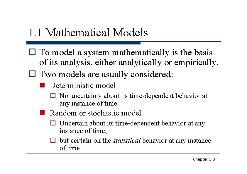
1. 1 Mathematical Models To model a system mathematically is the basis of its analysis, either analytically or empirically. Two models are usually considered: Deterministic model No uncertainty about its time-dependent behavior at any instance of time. Random or stochastic model Uncertain about its time-dependent behavior at any instance of time, but certain on the statistical behavior at any instance of time. Chapter 1 -3

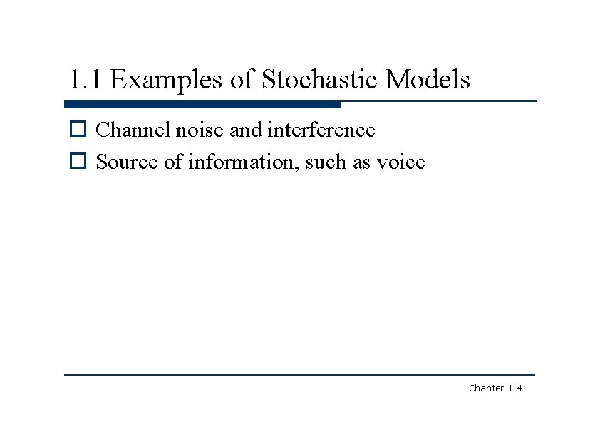
1. 1 Examples of Stochastic Models Channel noise and interference Source of information, such as voice Chapter 1 -4

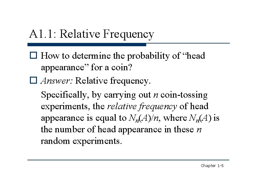
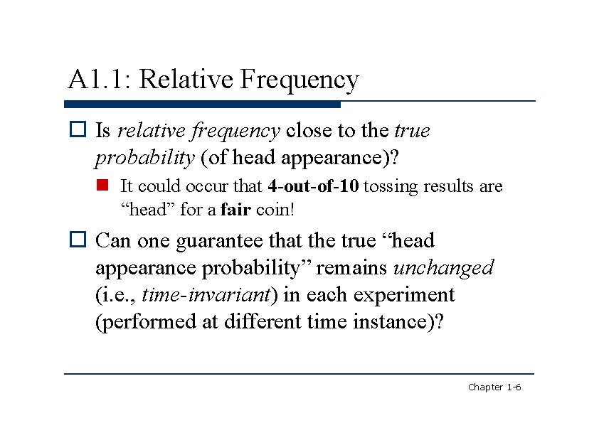
A 1. 1: Relative Frequency How to determine the probability of “head appearance” for a coin? Answer: Relative frequency. Specifically, by carrying out n coin-tossing experiments, the relative frequency of head appearance is equal to Nn(A)/n, where Nn(A) is the number of head appearance in these n random experiments. Chapter 1 -5

A 1. 1: Relative Frequency Is relative frequency close to the true probability (of head appearance)? It could occur that 4 -out-of-10 tossing results are “head” for a fair coin! Can one guarantee that the true “head appearance probability” remains unchanged (i. e. , time-invariant) in each experiment (performed at different time instance)? Chapter 1 -6

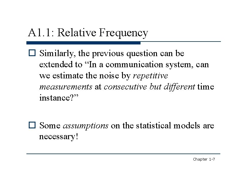
A 1. 1: Relative Frequency Similarly, the previous question can be extended to “In a communication system, can we estimate the noise by repetitive measurements at consecutive but different time instance? ” Some assumptions on the statistical models are necessary! Chapter 1 -7

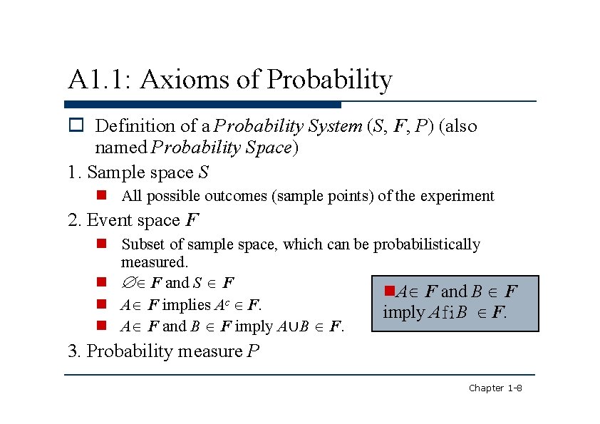
A 1. 1: Axioms of Probability Definition of a Probability System (S, F, P) (also named Probability Space) 1. Sample space S All possible outcomes (sample points) of the experiment 2. Event space F Subset of sample space, which can be probabilistically measured. F and S F A F and B F c A F implies A F. imply A f i B F. A F and B F imply A∪B F. 3. Probability measure P Chapter 1 -8

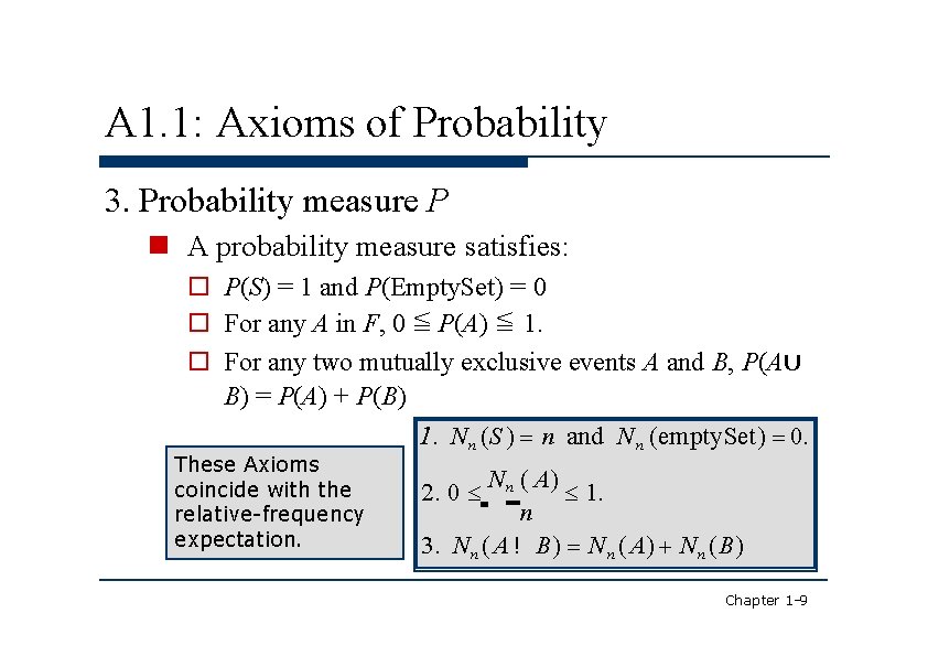
A 1. 1: Axioms of Probability 3. Probability measure P A probability measure satisfies: P(S) = 1 and P(Empty. Set) = 0 For any A in F, 0 ≦ P(A) ≦ 1. For any two mutually exclusive events A and B, P(A∪ B) = P(A) + P(B) 1. N n (S ) n and N n (empty. Set) 0. These Axioms coincide with the relative-frequency expectation. N n ( A) 1. n 3. N n ( A ! B) N n ( A) N n (B) 2. 0 Chapter 1 -9

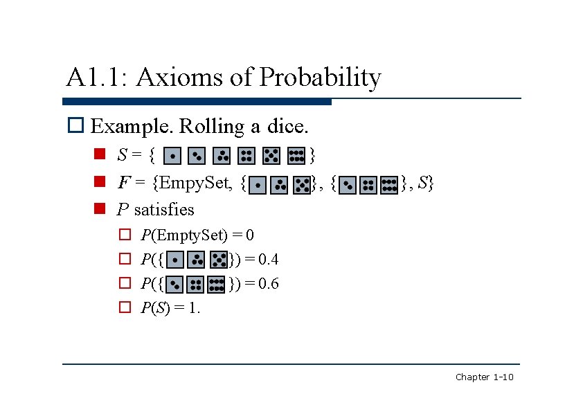
A 1. 1: Axioms of Probability Example. Rolling a dice. S={ F = {Empy. Set, { P satisfies } }, { }, S} P(Empty. Set) = 0 P({ }) = 0. 4 P({ }) = 0. 6 P(S) = 1. Chapter 1 -10

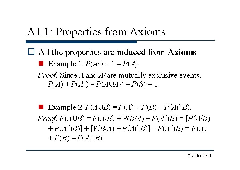
A 1. 1: Properties from Axioms All the properties are induced from Axioms Example 1. P(Ac) = 1 – P(A). Proof. Since A and Ac are mutually exclusive events, P(A) + P(Ac) = P(A∪Ac) = P(S) = 1. Example 2. P(A∪B) = P(A) + P(B) – P(A∩B). Proof. P(A∪B) = P(A/B) + P(B/A) + P(A∩B) = [P(A/B) + P(A∩B)] + [P(B/A) + P(A∩B)] – P(A∩B) = P(A) + P(B) – P(A∩B). Chapter 1 -11

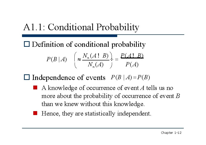
A 1. 1: Conditional Probability Definition of conditional probability P(B | A) N n ( A ! B) P( A) N n ( A) Independence of events P(B | A) P(B) A knowledge of occurrence of event A tells us no more about the probability of occurrence of event B than we knew without this knowledge. Hence, they are statistically independent. Chapter 1 -12

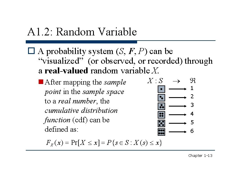
A 1. 2: Random Variable A probability system (S, F, P) can be “visualized” (or observed, or recorded) through a real-valued random variable X. After mapping the sample point in the sample space to a real number, the cumulative distribution function (cdf) can be defined as: X : S 1 2 3 4 5 6 FX ( x) Pr[ X x] P{s S : X (s) x} Chapter 1 -13

A 1. 2: Random Variable Since the event [X ≦ x] has to be probabilistically measurable for any real number x, the event space F must consist of all the elements of the form [X ≦ x]. In previous example, the event space F must contain the intersections and unions of the following 6 sets. }={s S: X(s)≦ 1} Otherwise, the cdf is { }={s S: X(s)≦ 2} not well-defined. { { }={s S: X(s)≦ 3} { }={s S: X(s)≦ 4} { }={s S: X(s)≦ 5} { }={s S: X(s)≦ 6} Chapter 1 -14

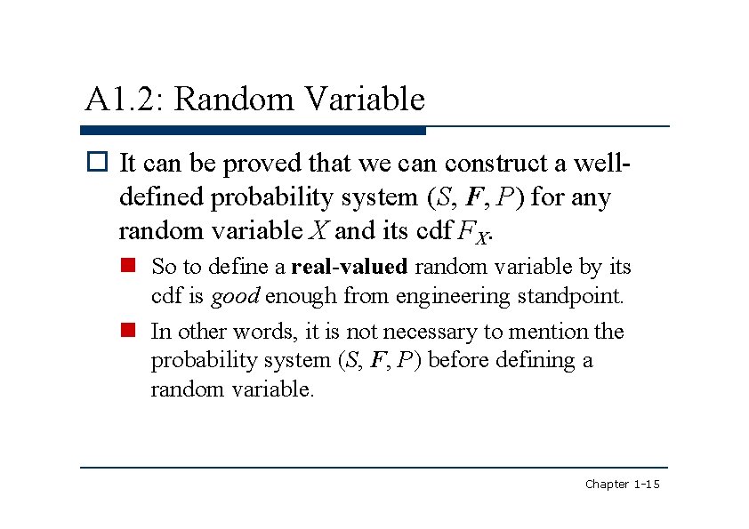
A 1. 2: Random Variable It can be proved that we can construct a welldefined probability system (S, F, P) for any random variable X and its cdf FX. So to define a real-valued random variable by its cdf is good enough from engineering standpoint. In other words, it is not necessary to mention the probability system (S, F, P) before defining a random variable. Chapter 1 -15

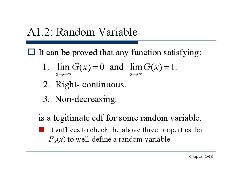
A 1. 2: Random Variable It can be proved that any function satisfying: 1. lim G(x) 0 and lim G(x) 1. x x 2. Right- continuous. 3. Non-decreasing. is a legitimate cdf for some random variable. It suffices to check the above three properties for FX(x) to well-define a random variable. Chapter 1 -16

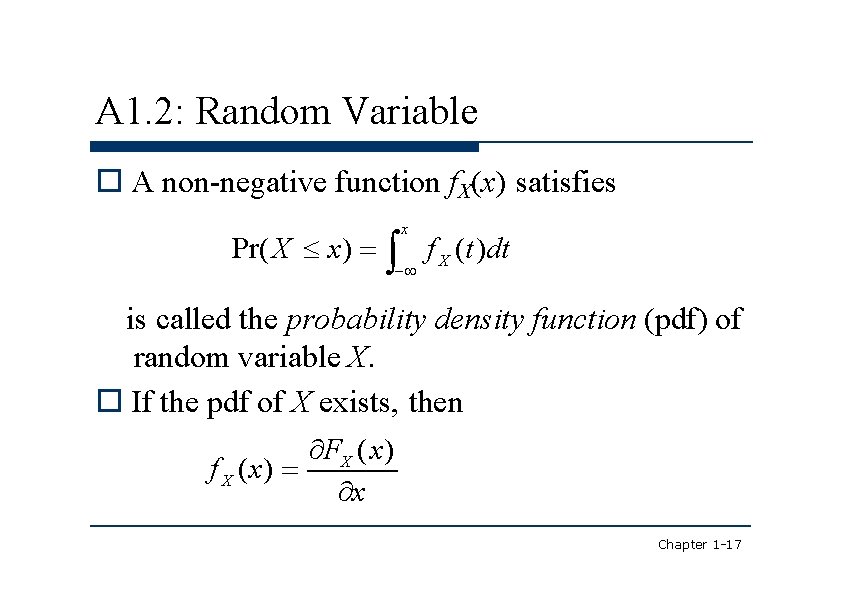
A 1. 2: Random Variable A non-negative function f. X(x) satisfies Pr( X x) x f X (t)dt is called the probability density function (pdf) of random variable X. If the pdf of X exists, then FX ( x) f X ( x) x Chapter 1 -17

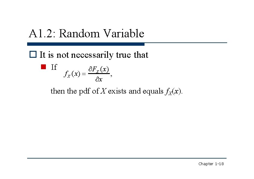
A 1. 2: Random Variable It is not necessarily true that If FX ( x) f X ( x) , x then the pdf of X exists and equals f. X(x). Chapter 1 -18

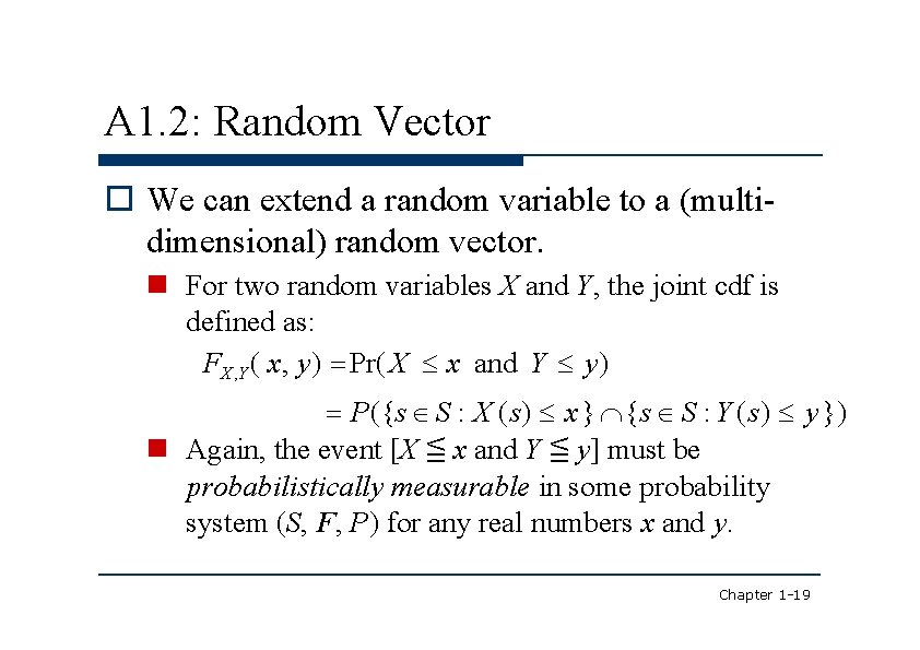
A 1. 2: Random Vector We can extend a random variable to a (multidimensional) random vector. For two random variables X and Y, the joint cdf is defined as: FX , Y ( x, y) Pr( X x and Y y) P({s S : X (s) x } {s S : Y (s) y }) Again, the event [X ≦ x and Y ≦ y] must be probabilistically measurable in some probability system (S, F, P) for any real numbers x and y. Chapter 1 -19

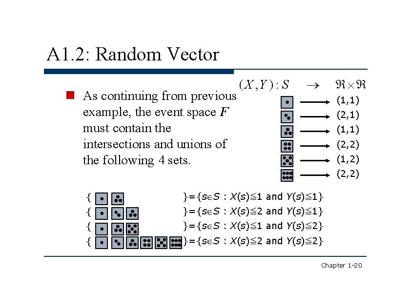
A 1. 2: Random Vector As continuing from previous example, the event space F must contain the intersections and unions of the following 4 sets. ( X , Y ) : S (1, 1) (2, 1) (1, 1) (2, 2) (1, 2) (2, 2) { }={s S : X(s)≦ 1 and Y(s)≦ 1} { }={s S : X(s)≦ 2 and Y(s)≦ 1} { }={s S : X(s)≦ 1 and Y(s)≦ 2} { }={s S : X(s)≦ 2 and Y(s)≦ 2} Chapter 1 -20

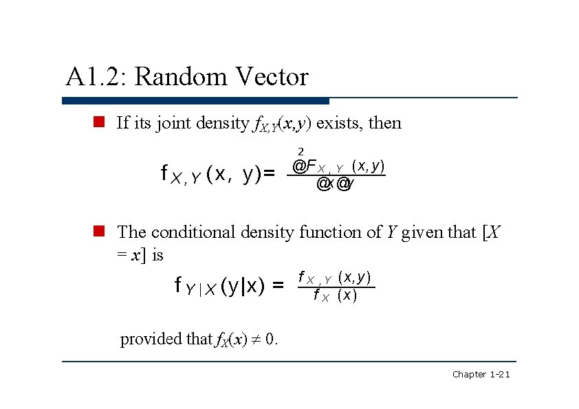
A 1. 2: Random Vector If its joint density f. X, Y(x, y) exists, then f X , Y ( x , y) = 2 @F X , Y (x, y) @x @y The conditional density function of Y given that [X = x] is f Y | X (y|x) = f X , Y (x, y) f X (x) provided that f. X(x) 0. Chapter 1 -21

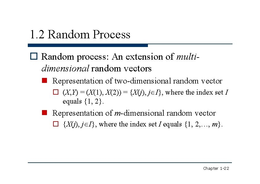
1. 2 Random Process Random process: An extension of multidimensional random vectors Representation of two-dimensional random vector (X, Y) = (X(1), X(2)) = {X(j), j I}, where the index set I equals {1, 2}. Representation of m-dimensional random vector {X(j), j I}, where the index set I equals {1, 2, …, m}. Chapter 1 -22

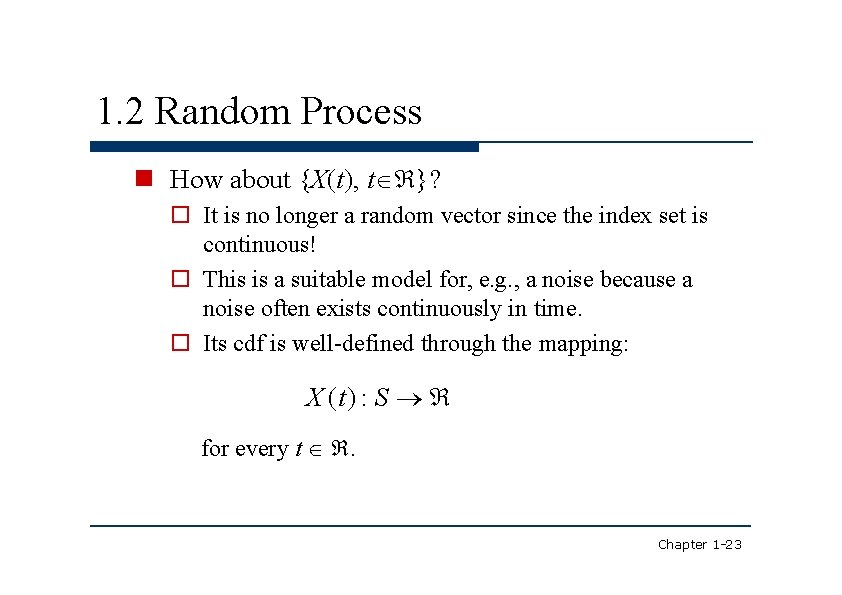
1. 2 Random Process How about {X(t), t }? It is no longer a random vector since the index set is continuous! This is a suitable model for, e. g. , a noise because a noise often exists continuously in time. Its cdf is well-defined through the mapping: X (t) : S for every t . Chapter 1 -23

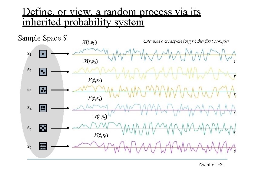
Define, or view, a random process via its inherited probability system Sample Space S X(t, s 1) outcome corresponding to the first sample s 1 t X(t, s 2) s 2 t X(t, s 3) s 3 t X(t, s 4) s 4 t X(t, s 5) s 5 t X(t, s 6) s 6 t Chapter 1 -24

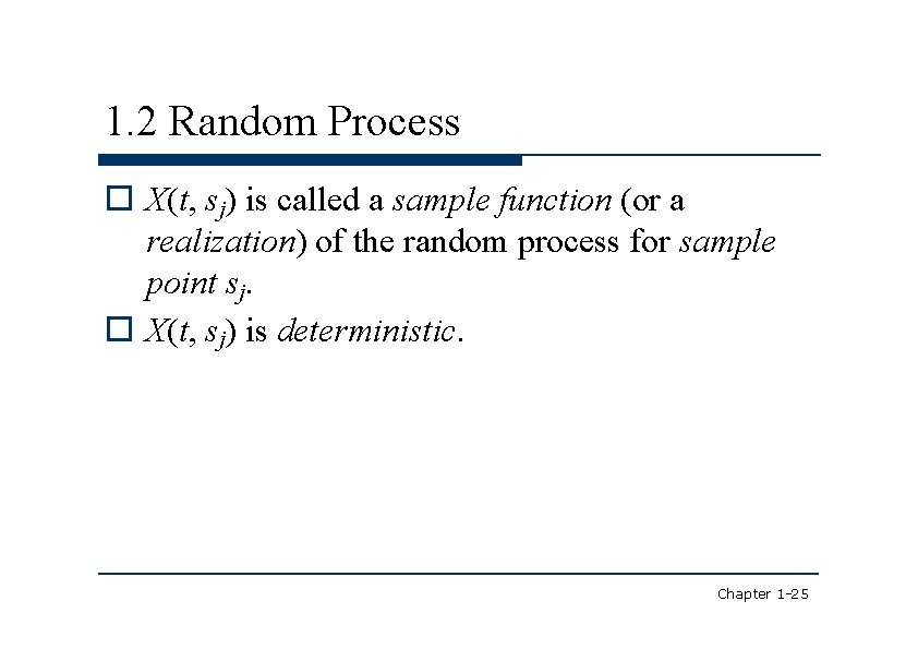
1. 2 Random Process X(t, sj) is called a sample function (or a realization) of the random process for sample point sj. X(t, sj) is deterministic. Chapter 1 -25

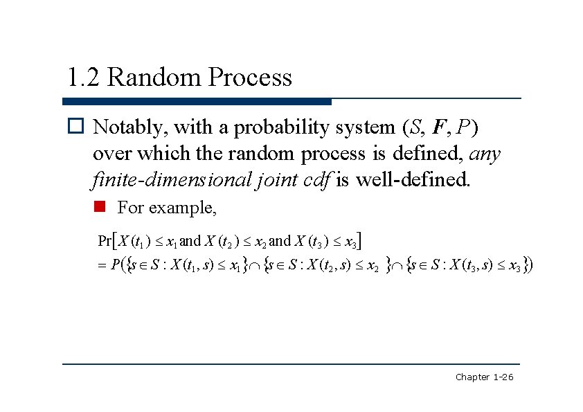
1. 2 Random Process Notably, with a probability system (S, F, P) over which the random process is defined, any finite-dimensional joint cdf is well-defined. For example, Pr X (t 1 ) x 1 and X (t 2 ) x 2 and X (t 3 ) x 3 P s S : X (t 1 , s) x 1 s S : X (t 2 , s) x 2 s S : X (t 3, s) x 3 Chapter 1 -26

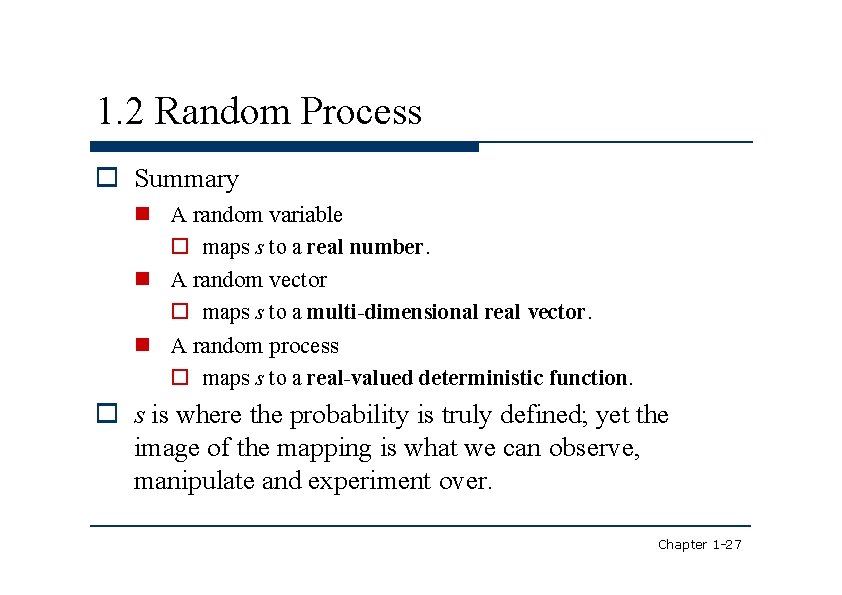
1. 2 Random Process Summary A random variable maps s to a real number. A random vector maps s to a multi-dimensional real vector. A random process maps s to a real-valued deterministic function. s is where the probability is truly defined; yet the image of the mapping is what we can observe, manipulate and experiment over. Chapter 1 -27