Information Retrieval continued Many slides in this presentation

Information Retrieval continued Many slides in this presentation are from Christopher D. Manning, Prabhakar Raghavan and Hinrich Schütze, Introduction to Information Retrieval, Cambridge University Press. 2008. Book available online at http: //nlp. stanford. edu/IRbook/information-retrieval-book. html

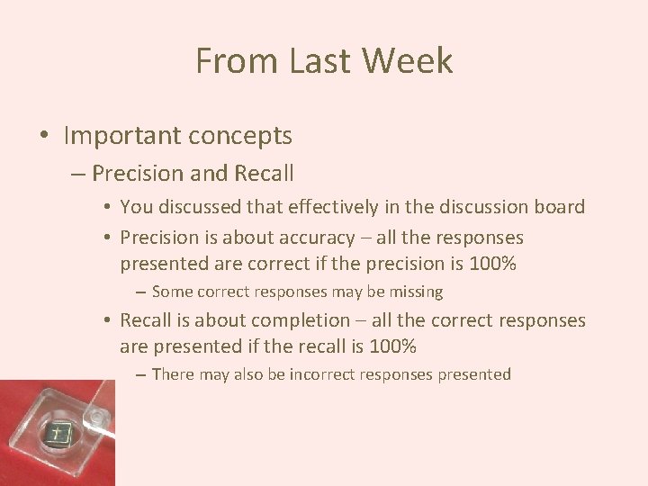
From Last Week • Important concepts – Precision and Recall • You discussed that effectively in the discussion board • Precision is about accuracy – all the responses presented are correct if the precision is 100% – Some correct responses may be missing • Recall is about completion – all the correct responses are presented if the recall is 100% – There may also be incorrect responses presented

Stop and think • If you had to choose between precision and recall, which would you choose? • Give an example when each would be preferable. Everyone, provide an example of each. Everyone, comment on an example of each provided by someone else. – Ideally, do this in real time. However, you may need to come back to do your comments after others have finished. Some discussion last week, but not conclusive. Discuss now.

Discuss • What was the best example of precision as being more important? • What was the best example of recall being more important? • Try to come to consensus in your discussion. I did not see this in the discussions

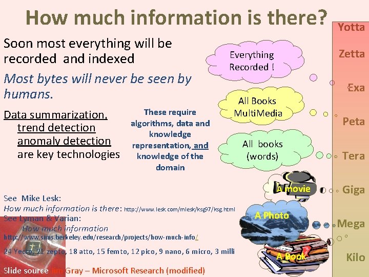
How much information is there? Soon most everything will be recorded and indexed Most bytes will never be seen by humans. Data summarization, trend detection anomaly detection are key technologies These require algorithms, data and knowledge representation, and knowledge of the domain Zetta Everything Recorded ! All Books Multi. Media See Mike Lesk: How much information is there: http: //www. lesk. com/mlesk/ksg 97/ksg. html See Lyman & Varian: How much information Yotta All books (words) A movie A Photo Exa Peta Tera Giga Mega http: //www. sims. berkeley. edu/research/projects/how-much-info/ 24 Yecto, 21 zepto, 18 atto, 15 femto, 12 pico, 9 nano, 6 micro, 3 milli Slide source Jim Gray – Microsoft Research (modified) A Book Kilo

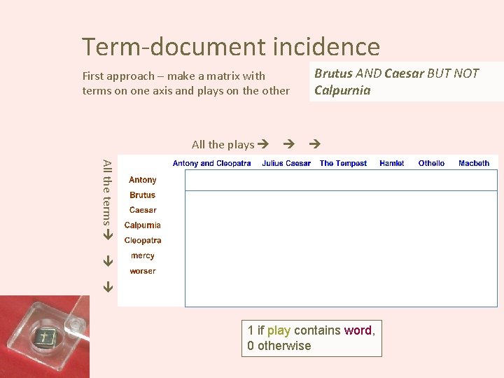
Term-document incidence First approach – make a matrix with terms on one axis and plays on the other All the plays Brutus AND Caesar BUT NOT Calpurnia All the terms 1 if play contains word, 0 otherwise

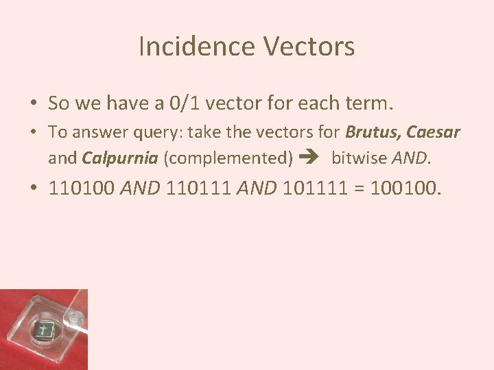
Incidence Vectors • So we have a 0/1 vector for each term. • To answer query: take the vectors for Brutus, Caesar and Calpurnia (complemented) bitwise AND. • 110100 AND 110111 AND 101111 = 100100.

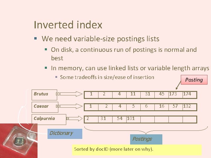
Inverted index § We need variable-size postings lists § On disk, a continuous run of postings is normal and best § In memory, can use linked lists or variable length arrays § Some tradeoffs in size/ease of insertion Brutus 1 Caesar 1 Calpurnia Dictionary 2 2 2 31 Posting 4 11 31 45 173 4 5 6 16 174 57 132 54 101 Postings Sorted by doc. ID (more later on why). 8

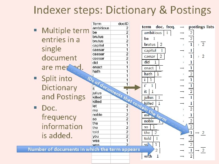
Indexer steps: Dictionary & Postings § Multiple term entries in a single document are merged. IDs § Split into of do cum Dictionary ent s th and Postings at con tai nt § Doc. he ter m frequency information is added. Number of documents in which the term appears

Query-document matching scores • We need a way of assigning a score to a query/document pair • Let’s start with a one-term query • If the query term does not occur in the document: score should be 0 • The more frequent the query term in the document, the higher the score (should be) • We will look at a number of alternatives for this.

Take 1: Jaccard coefficient • A commonly used measure of overlap of two sets A and B – jaccard(A, B) = |A ∩ B| / |A ∪ B| – jaccard(A, A) = 1 – jaccard(A, B) = 0 if A ∩ B = 0 • A and B don’t have to be the same size. • Always assigns a number between 0 and 1.

Issues with Jaccard for scoring • It doesn’t consider term frequency (how many times a term occurs in a document) – Rare terms in a collection are more informative than frequent terms. Jaccard doesn’t consider this information • We need a more sophisticated way of normalizing for length The problem with the first example was that document 2 “won” because it was shorter, not because it was a better match. We need a way to take into account document length so that longer documents are not penalized in calculating the match score.

Spot check • Compute the Jaccard coefficients for this example: • Query: Computer Course • Document 1: Computer Science Courses for Everyone; Fall 2012 offerings from the CSC Department with no prerequisites • Document 2: Blown to Bits -- course on technology impact

Recall : Binary term-document incidence matrix Each document is represented by a binary vector ∈ {0, 1}|V|

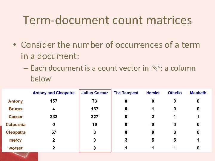
Term-document count matrices • Consider the number of occurrences of a term in a document: – Each document is a count vector in ℕv: a column below

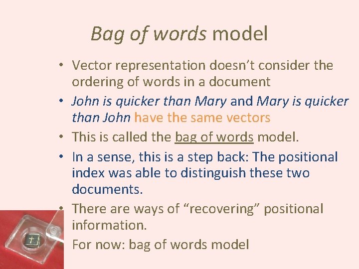
Bag of words model • Vector representation doesn’t consider the ordering of words in a document • John is quicker than Mary and Mary is quicker than John have the same vectors • This is called the bag of words model. • In a sense, this is a step back: The positional index was able to distinguish these two documents. • There are ways of “recovering” positional information. • For now: bag of words model

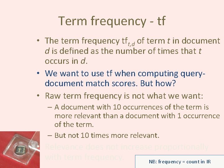
Term frequency - tf • The term frequency tft, d of term t in document d is defined as the number of times that t occurs in d. • We want to use tf when computing querydocument match scores. But how? • Raw term frequency is not what we want: – A document with 10 occurrences of the term is more relevant than a document with 1 occurrence of the term. – But not 10 times more relevant. • Relevance does not increase proportionally with term frequency. NB: frequency = count in IR

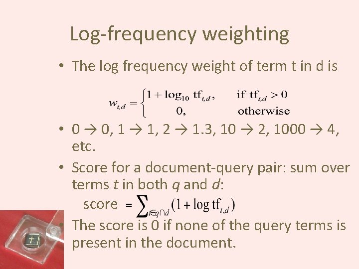
Log-frequency weighting • The log frequency weight of term t in d is • 0 → 0, 1 → 1, 2 → 1. 3, 10 → 2, 1000 → 4, etc. • Score for a document-query pair: sum over terms t in both q and d: score • The score is 0 if none of the query terms is present in the document.

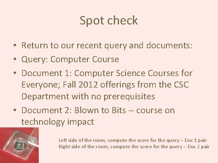
Spot check • Return to our recent query and documents: • Query: Computer Course • Document 1: Computer Science Courses for Everyone; Fall 2012 offerings from the CSC Department with no prerequisites • Document 2: Blown to Bits -- course on technology impact Left side of the room, compute the score for the query – Doc 1 pair Right side of the room, compute the score for the query – Doc 2 pair

Document frequency • Rare terms are more informative than frequent terms – Recall stop words • Consider a term in the query that is rare in the collection (e. g. , arachnocentric) • A document containing this term is very likely to be relevant to the query arachnocentric • → We want a high weight for rare terms like arachnocentric, even if the term does not appear many times in the document.

Document frequency, continued • Frequent terms are less informative than rare terms • Consider a query term that is frequent in the collection (e. g. , high, increase, line) – A document containing such a term is more likely to be relevant than a document that doesn’t – But it’s not a sure indicator of relevance. • → For frequent terms, we want high positive weights for words like high, increase, and line – But lower weights than for rare terms. • We will use document frequency (df) to capture this.

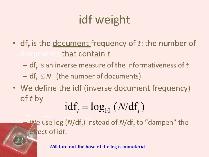
idf weight • dft is the document frequency of t: the number of documents that contain t – dft is an inverse measure of the informativeness of t – dft N (the number of documents) • We define the idf (inverse document frequency) of t by – We use log (N/dft) instead of N/dft to “dampen” the effect of idf. Will turn out the base of the log is immaterial.

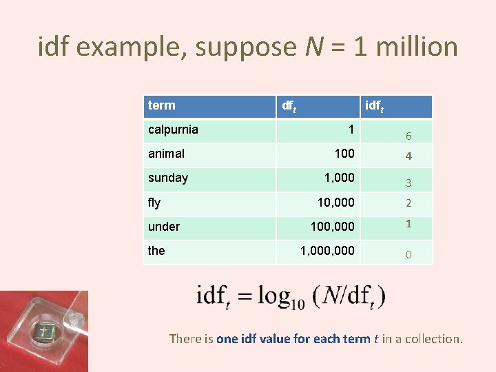
idf example, suppose N = 1 million term calpurnia dft idft 1 6 animal 100 4 sunday 1, 000 3 10, 000 2 100, 000 1 1, 000 0 fly under the There is one idf value for each term t in a collection.

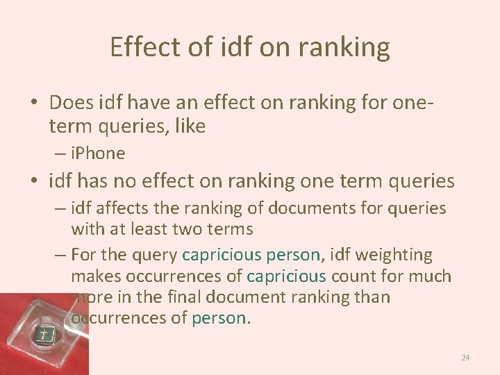
Effect of idf on ranking • Does idf have an effect on ranking for oneterm queries, like – i. Phone • idf has no effect on ranking one term queries – idf affects the ranking of documents for queries with at least two terms – For the query capricious person, idf weighting makes occurrences of capricious count for much more in the final document ranking than occurrences of person. 24

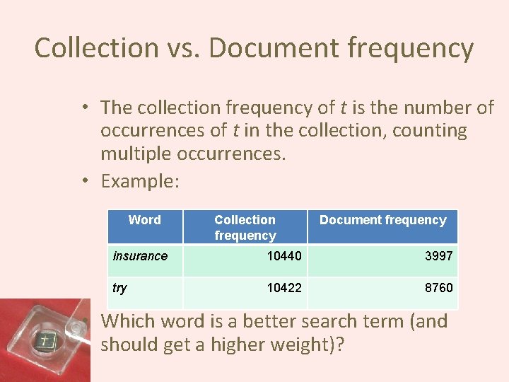
Collection vs. Document frequency • The collection frequency of t is the number of occurrences of t in the collection, counting multiple occurrences. • Example: Word Collection frequency Document frequency insurance 10440 3997 try 10422 8760 • Which word is a better search term (and should get a higher weight)?

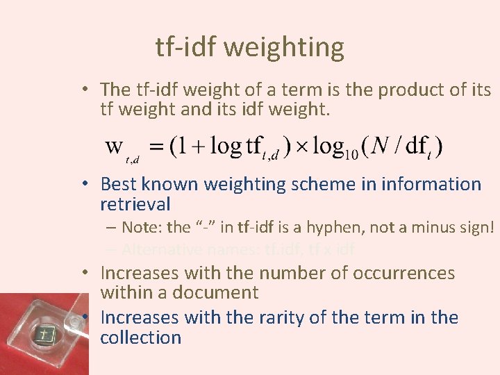
tf-idf weighting • The tf-idf weight of a term is the product of its tf weight and its idf weight. • Best known weighting scheme in information retrieval – Note: the “-” in tf-idf is a hyphen, not a minus sign! – Alternative names: tf. idf, tf x idf • Increases with the number of occurrences within a document • Increases with the rarity of the term in the collection

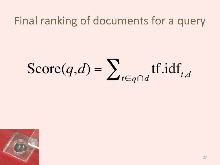
Final ranking of documents for a query 27

Spot Check • Go back to our example from the Spot Check on Jaccard. Compute the tf-idf score for the query relative to each of the documents. – Query: Computer Course – Document 1: Computer Science Courses for Everyone; Fall 2012 offerings from the CSC Department with no prerequisites – Document 2: Blown to Bits -- course on technology impact • The example is so small it is hard to see the effect, but do you see any difference between this and the Jaccard index?

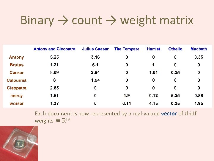
Binary → count → weight matrix Each document is now represented by a real-valued vector of tf-idf weights ∈ R|V|

Documents as vectors • • So we have a |V|-dimensional vector space Terms are axes of the space Documents are points or vectors in this space Very high-dimensional: tens of millions of dimensions when you apply this to a web search engine These are very sparse vectors - most entries are zero.

Spot check • In your usual groupings, – Find at least three news articles on some recent event (earthquakes, fires, Santorum, etc. ) – Take the first two sentences of each article and make that the document. You now have three documents. – Form the vector of all the words from all the documents. – Show the vector for each of the documents • This vector will have the count of the number of times the corresponding word appears in this document. Start with counts. Then turn into tf-idf weights.

Queries as vectors • Key idea 1: Do the same for queries: represent them as vectors in the space • Key idea 2: Rank documents according to their proximity to the query in this space • proximity = similarity of vectors • proximity ≈ inverse of distance • Recall: We do this because we want to get away from the you’re-either-in-or-out Boolean model. • Instead: rank more relevant documents higher than less relevant documents

Formalizing vector space proximity • First cut: distance between two points ( = distance between the end points of the two vectors) • Euclidean distance? • Euclidean distance is a bad idea. . . • . . . because Euclidean distance is large for vectors of different lengths.

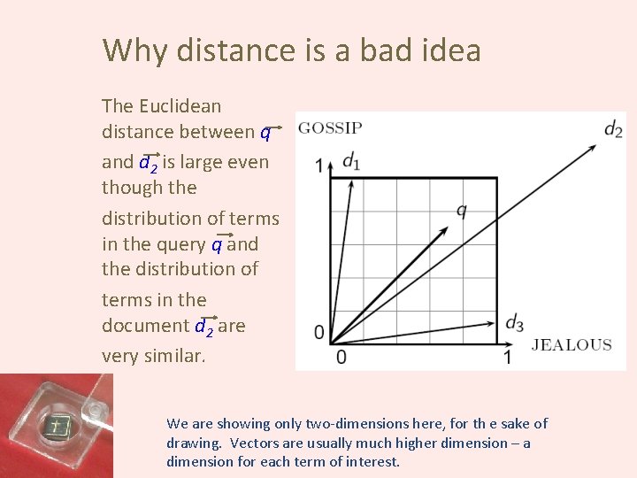
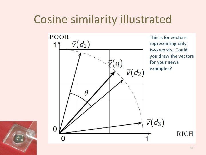
Why distance is a bad idea The Euclidean distance between q and d 2 is large even though the distribution of terms in the query q and the distribution of terms in the document d 2 are very similar. We are showing only two-dimensions here, for th e sake of drawing. Vectors are usually much higher dimension – a dimension for each term of interest.

Use angle instead of distance • Thought experiment: take a document d and append it to itself. Call this document d′. • “Semantically” d and d′ have the same content • The Euclidean distance between the two documents can be quite large • The angle between the two documents is 0, corresponding to maximal similarity. • Key idea: Rank documents according to angle with query.

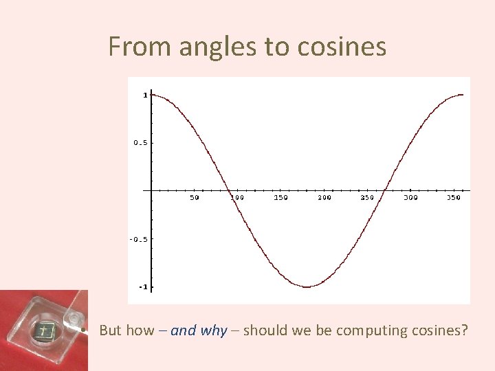
From angles to cosines • The following two notions are equivalent. – Rank documents in decreasing order of the angle between query and document – Rank documents in increasing order of cosine(query, document) • Cosine is a monotonically decreasing function for the interval [0 o, 180 o] Therefore, a small angle results in a large cosine and a large angle results in a small cosine – just the behavior we need.

From angles to cosines • But how – and why – should we be computing cosines?

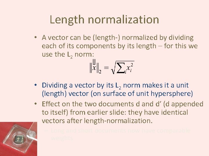
Length normalization • A vector can be (length-) normalized by dividing each of its components by its length – for this we use the L 2 norm: • Dividing a vector by its L 2 norm makes it a unit (length) vector (on surface of unit hypersphere) • Effect on the two documents d and d′ (d appended to itself) from earlier slide: they have identical vectors after length-normalization. – Long and short documents now have comparable weights

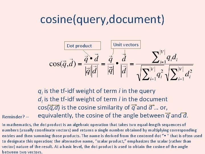
cosine(query, document) Dot product Reminder? -- Unit vectors qi is the tf-idf weight of term i in the query di is the tf-idf weight of term i in the document cos(q, d) is the cosine similarity of q and d … or, equivalently, the cosine of the angle between q and d. In mathematics, the dot product is an algebraic operation that takes two equal-length sequences of numbers (usually coordinate vectors) and returns a single number obtained by multiplying corresponding entries and then summing those products. The name is derived from the centered dot ” " that is often used to designate this operation; the alternative name, “scalar product, ” emphasizes the scalar (rather than vector) nature of the result. At a basic level, the dot product is used to obtain the cosine of the angle between two vectors.

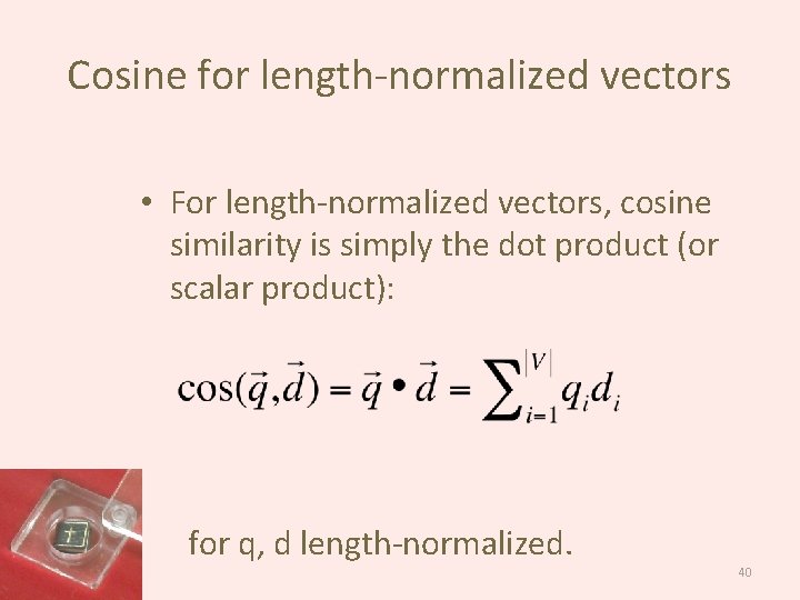
Cosine for length-normalized vectors • For length-normalized vectors, cosine similarity is simply the dot product (or scalar product): for q, d length-normalized. 40

Cosine similarity illustrated This is for vectors representing only two words. Could you draw the vectors for your news examples? 41

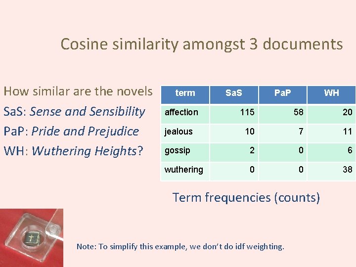
Cosine similarity amongst 3 documents How similar are the novels Sa. S: Sense and Sensibility Pa. P: Pride and Prejudice WH: Wuthering Heights? term affection Sa. S Pa. P WH 115 58 20 jealous 10 7 11 gossip 2 0 6 wuthering 0 0 38 Term frequencies (counts) Note: To simplify this example, we don’t do idf weighting.

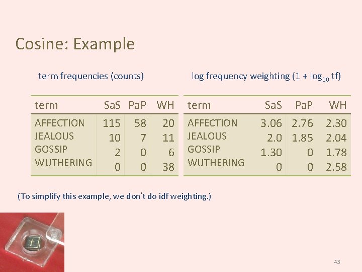
Cosine: Example term frequencies (counts) term Sa. S Pa. P WH AFFECTION 115 58 20 JEALOUS 10 7 11 GOSSIP 2 0 6 WUTHERING 0 0 38 log frequency weighting (1 + log 10 tf) term AFFECTION JEALOUS GOSSIP WUTHERING Sa. S Pa. P 3. 06 2. 76 2. 0 1. 85 1. 30 0 WH 2. 30 2. 04 1. 78 2. 58 (To simplify this example, we don't do idf weighting. ) 43 43

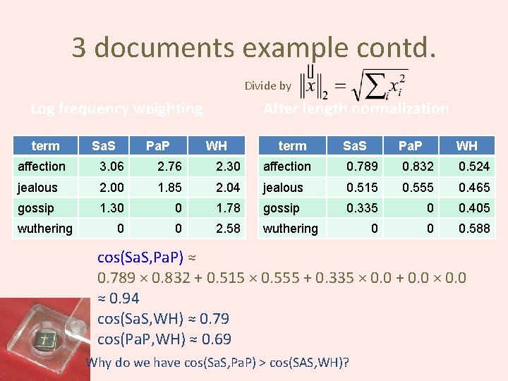
3 documents example contd. Divide by Log frequency weighting term Sa. S Pa. P After length normalization WH term Sa. S Pa. P WH affection 3. 06 2. 76 2. 30 affection 0. 789 0. 832 0. 524 jealous 2. 00 1. 85 2. 04 jealous 0. 515 0. 555 0. 465 gossip 1. 30 0 1. 78 gossip 0. 335 0 0. 405 0 0 2. 58 wuthering 0 0 0. 588 wuthering cos(Sa. S, Pa. P) ≈ 0. 789 × 0. 832 + 0. 515 × 0. 555 + 0. 335 × 0. 0 + 0. 0 × 0. 0 ≈ 0. 94 cos(Sa. S, WH) ≈ 0. 79 cos(Pa. P, WH) ≈ 0. 69 Why do we have cos(Sa. S, Pa. P) > cos(SAS, WH)?

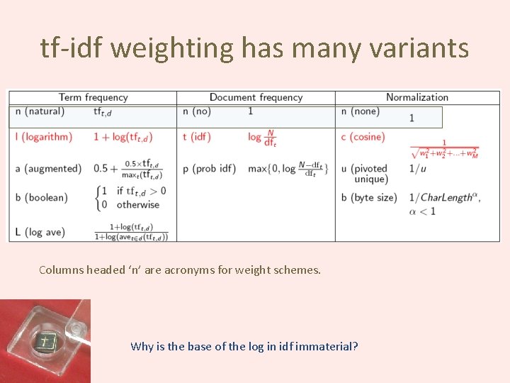
tf-idf weighting has many variants Columns headed ‘n’ are acronyms for weight schemes. Why is the base of the log in idf immaterial?

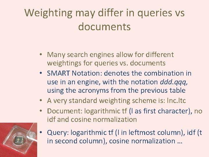
Weighting may differ in queries vs documents • Many search engines allow for different weightings for queries vs. documents • SMART Notation: denotes the combination in use in an engine, with the notation ddd. qqq, using the acronyms from the previous table • A very standard weighting scheme is: lnc. ltc • Document: logarithmic tf (l as first character), no idf and cosine normalization • Query: logarithmic tf (l in leftmost column), idf (t in second column), cosine normalization …

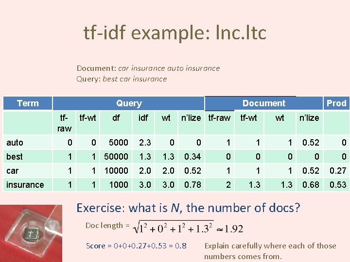
tf-idf example: lnc. ltc Document: car insurance auto insurance Query: best car insurance Term Query tf-wt raw df idf Document wt n’lize tf-raw tf-wt Prod wt n’lize auto 0 0 5000 2. 3 0 0 1 1 1 0. 52 0 best 1 1 50000 1. 3 0. 34 0 0 0 car 1 1 10000 2. 0 0. 52 1 1 1 0. 52 0. 27 insurance 1 1 3. 0 0. 78 2 1. 3 0. 68 0. 53 1000 Exercise: what is N, the number of docs? Doc length = Score = 0+0+0. 27+0. 53 = 0. 8 Explain carefully where each of those numbers comes from.

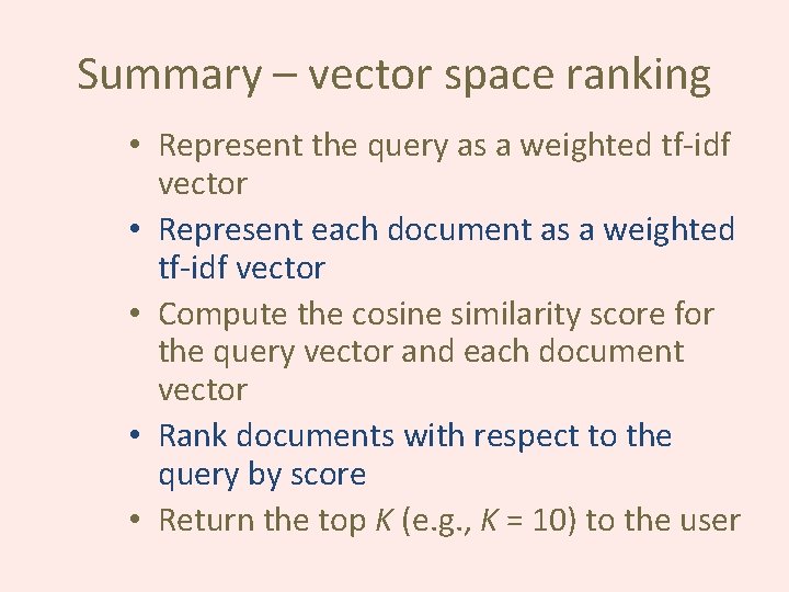
Summary – vector space ranking • Represent the query as a weighted tf-idf vector • Represent each document as a weighted tf-idf vector • Compute the cosine similarity score for the query vector and each document vector • Rank documents with respect to the query by score • Return the top K (e. g. , K = 10) to the user

A very important note • This is just the beginning • This is the basic theory of vector space modeling and term frequency weighting. • Spammers could easily fool this technique (and have done so). Real systems start with this and then do variations that attempt to defeat those who would cheat the system.

Resources for this lecture • Introduction to Information Retrieval, sections 6. 2 – 6. 4. 3 – Slides provided by the author • http: //www. miislita. com/informationretrieval-tutorial/cosine-similaritytutorial. html -- Term weighting and cosine similarity tutorial