Implementation of ICP Variants Pavan Ram Piratla Janani

Implementation of ICP Variants Pavan Ram Piratla Janani Venkateswaran

Outline • • Introduction Comparison Individual ICP stages Parameters for comparison Issues Conclusion Results

Introduction • • Implementation and comparison Original ICP algorithm Modified variant (more efficient) Algorithm modified in a couple of stages

Comparison • Besl and Mc. Kay [92] method for registering 3 D shapes • Based on iteratively finding the nearest point to a given point on a model • Variation based on a comparison paper by Rusinkiewicz and Levoy [ 2001]

Stages • • • Point selection Point matching Weighting Outlier removal Error metric Error minimization

Parameters • Random sampling of points on the surface • Most computationally expensive step: finding the closest point • n points : single point query complexity of O(n). • m samples: Complexity is O(mn) • The closest-point can be calculated with more efficiency by using other data structures like a kd tree or by caching

Octree • Efficient version: • Simplified implementation of an Octree • An octree works by subdividing the space into cubes

Octree Root node: Subdivided into 8 parts

Implementation • Using the octree, we can prune large areas without needing to consider them at all • When the cube we consider has no triangles, we disregard that section of the octree • Complexity is reduced drastically: the octree has a constant lookup time

Point-to-point matching • We perform closest-point matching by using a point-to-point metric • The ICP algorithm requires preprocessing to generate an octree • The 1 D representation accumulates information • Much faster than the initial ICP algorithm using octree

More Parameters • Weighting: Does not substantially affect performance • Rejection of outliers: Decreases speed and performance • Error metric: We use the l 2 distance as the error metric • Minimize the ε value at each iteration • Terminating condition: RMS residual error

Alternate issues • Speed increase using closest-point caching • If the termination threshold is small, caching significantly improves performance • Fastest surface point computation can be used

Advantages and disadvantages C Works much faster C Less computation D Requires preprocessing for the octree • Trade-off is worth it

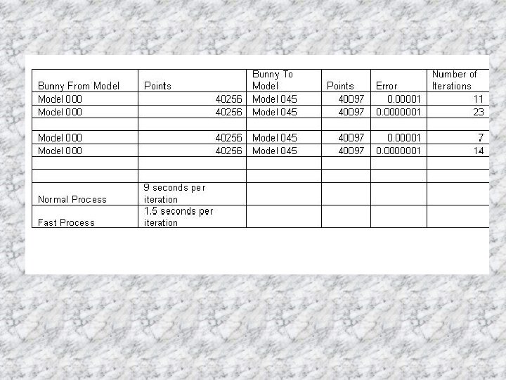
Results • Ran the iterations on the Stanford bunny • Used the simplified octree to find the closest point efficiently • Randomly sampled points on it • Iterations converge quickly • Results will be displayed at the end of the presentation

Bunny Model 000

Bunny Model 045

Bunny Model 0045

Bunny Model 0045 Fast

Bunny Model 4500

Conclusion • Compared the two algorithms • The efficiency in finding the closest point • Results show the iteration convergence and the lower computation required to perform it

References • Fast and Accurate Shape-based registration: David A. Simon http: //www. ri. cmu. edu/pub_files/pub 1/simon _david_1996_1/simon_david_1996_1. pdf • The Stanford 3 D scanning repository http: //graphics. stanford. edu/data/3 Dscanrep/ • http: //www. gametutorials. com/Tutorials/Op en. GL/Octree. htm

THANK YOU!