Personal Genomics Genotyping Shai Carmi School of Public

Personal Genomics Genotyping Shai Carmi School of Public Health

How to read genomes? • Traditional method: Sanger sequencing • Next generation sequencing • Microarrays

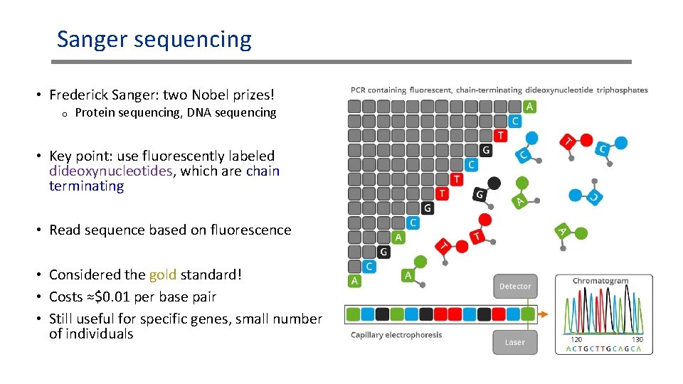
Sanger sequencing • Frederick Sanger: two Nobel prizes! o Protein sequencing, DNA sequencing • Key point: use fluorescently labeled dideoxynucleotides, which are chain terminating • Read sequence based on fluorescence • Considered the gold standard! • Costs ≈$0. 01 per base pair • Still useful for specific genes, small number of individuals

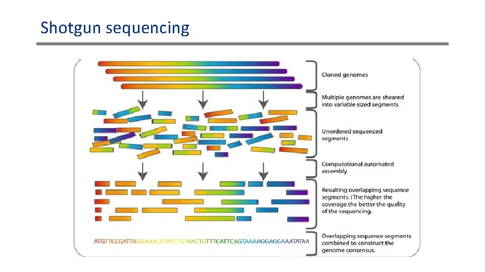
How to Sanger sequence entire genomes? • Sanger sequencing can only be applied to short fragments • How to sequence entire genomes? o Even bacterial or yeast, etc. • Idea: shotgun sequencing • Fragment (randomly) multiple copies of the genome into short segments (tens/hundreds of bp) • Sequence each fragment • Assemble the sequences into the entire genome

Shotgun sequencing

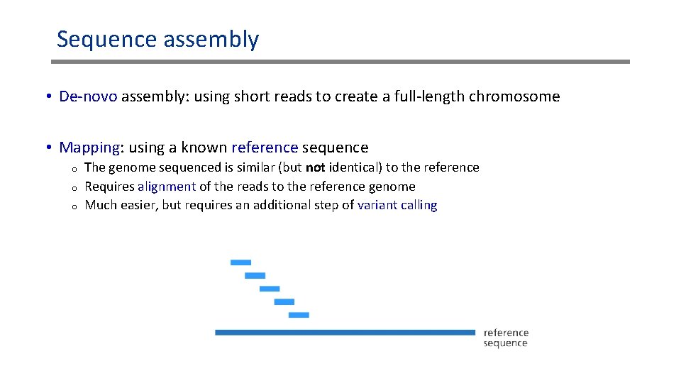
Sequence assembly • De-novo assembly: using short reads to create a full-length chromosome • Mapping: using a known reference sequence o o o The genome sequenced is similar (but not identical) to the reference Requires alignment of the reads to the reference genome Much easier, but requires an additional step of variant calling

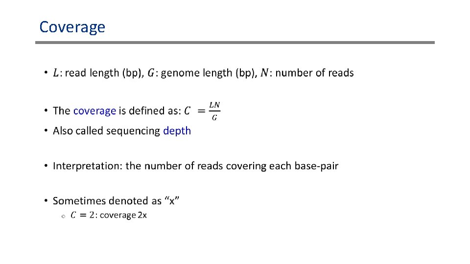
Coverage •

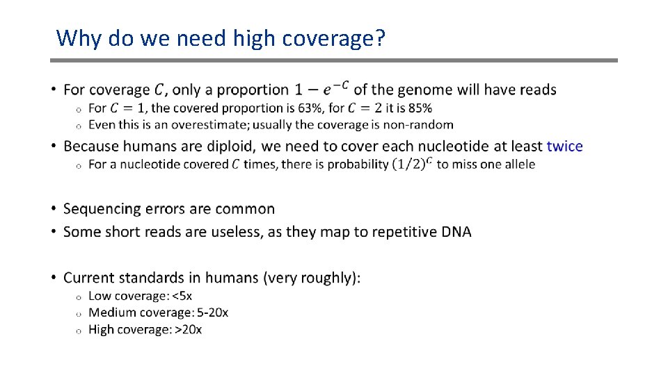
Why do we need high coverage? •

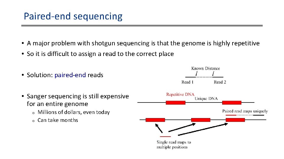
Paired-end sequencing • A major problem with shotgun sequencing is that the genome is highly repetitive • So it is difficult to assign a read to the correct place • Solution: paired-end reads • Sanger sequencing is still expensive for an entire genome o o Millions of dollars, even today Can take months

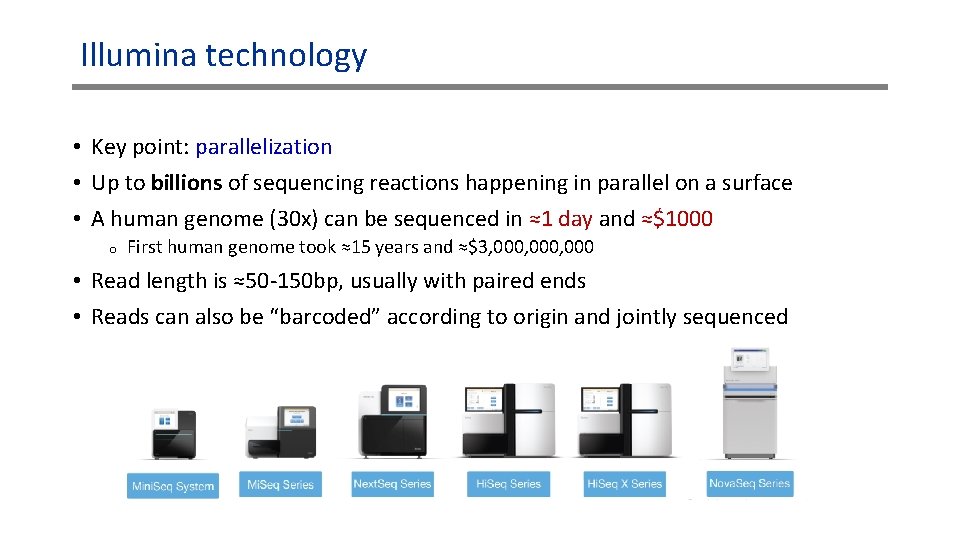
Illumina technology • Key point: parallelization • Up to billions of sequencing reactions happening in parallel on a surface • A human genome (30 x) can be sequenced in ≈1 day and ≈$1000 o First human genome took ≈15 years and ≈$3, 000, 000 • Read length is ≈50 -150 bp, usually with paired ends • Reads can also be “barcoded” according to origin and jointly sequenced

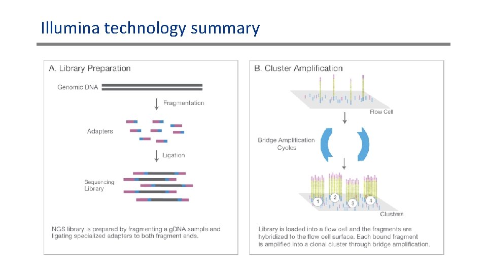
Illumina technology summary

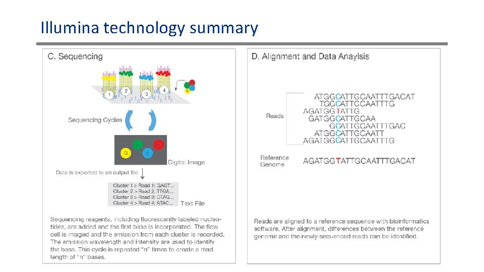
Illumina technology summary

Exome sequencing • For many applications, we care mostly about coding regions (exons) • Instead of sequencing the entire genome, we can sequence just ≈1 -2% of it o o o ≈30 -60 Mbp Due to the smaller target, the coverage is typically higher (≈100 x or more) Current cost around ≈$400 • Very useful for severe disorders, where the disease is likely monogenic and the causal mutation is likely coding • Currently very popular, but may go out of fashion due to the decrease in price of whole-genome sequencing (WGS) • It was shown that WGS is often more accurate even for coding regions o In particular for copy-number variants

Sequencing bioinformatics outline 1. Mapping reads to the reference genome (“alignment”) 2. Calling variants (differences from reference) 3. Quality control

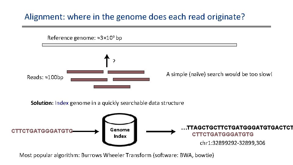
Alignment: where in the genome does each read originate? Reference genome: ≈3× 109 bp ? A simple (naïve) search would be too slow! Reads: ≈100 bp Solution: Index genome in a quickly searchable data structure CTTCTGATGGGATGTG Genome Index …TTAGCTGCTTCTGATGGGATGTGACTCT CTTCTGATGGGATGTG chr 1: 32899292 -32899, 306 Most popular algorithm: Burrows Wheeler Transform (software: BWA, bowtie)

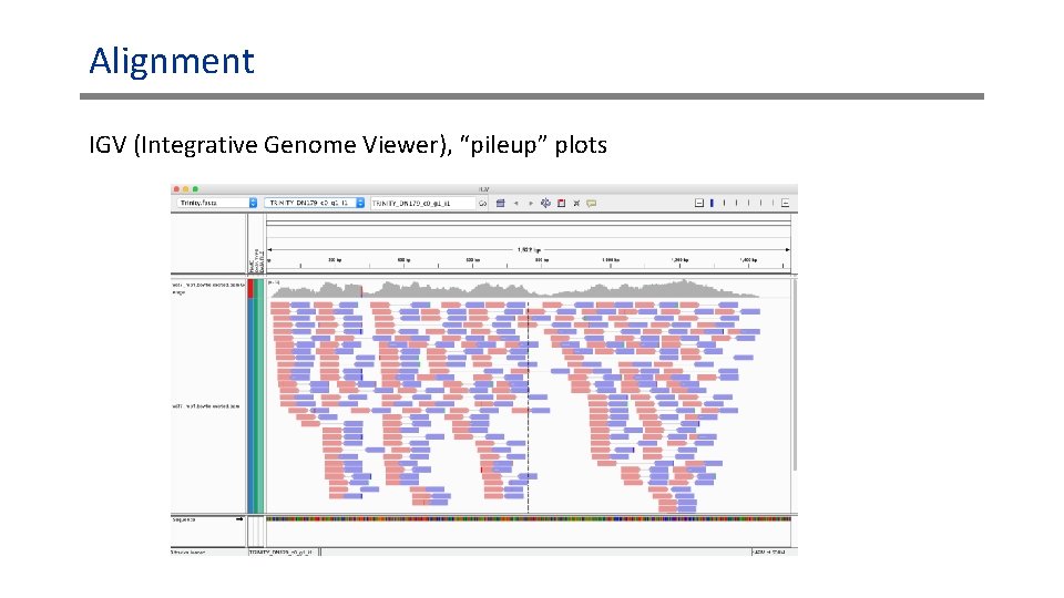
Alignment IGV (Integrative Genome Viewer), “pileup” plots

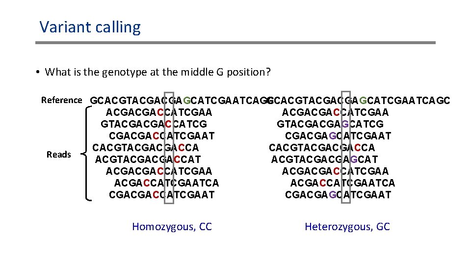
Variant calling • What is the genotype at the middle G position? Reference GCACGTACGACGAGCATCGAATCAGC ACGACGACCATCGAA GTACGACGACCATCG GTACGACGAGCATCG CGACGACCATCGAAT CGACGAGCATCGAAT CACGTACGACGACCA Reads ACGTACGACGACCAT ACGTACGACGAGCAT ACGACGACCATCGAATCA CGACGACCATCGAAT CGACGAGCATCGAAT Homozygous, CC Heterozygous, GC

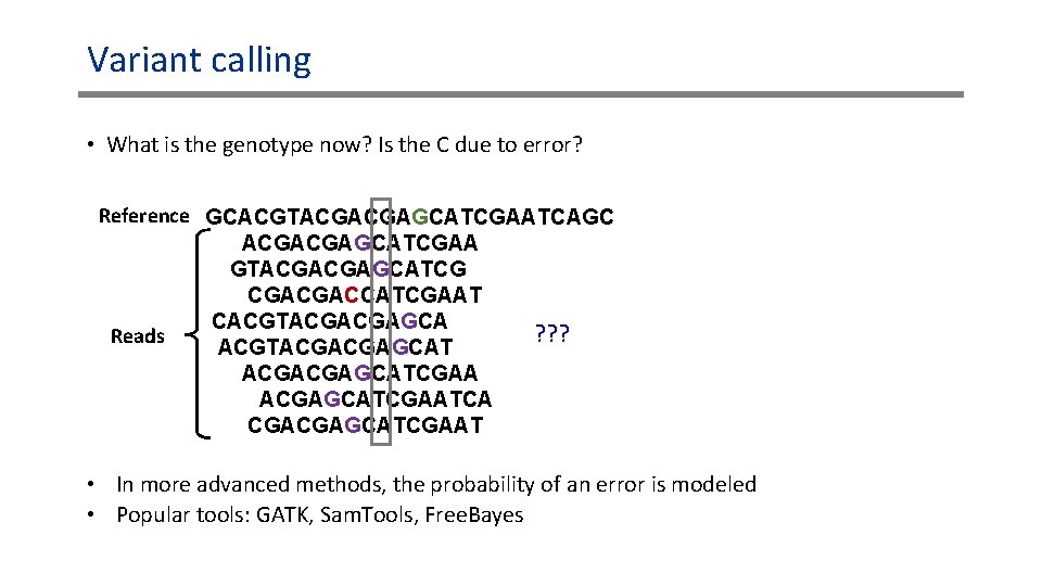
Variant calling • What is the genotype now? Is the C due to error? Reference GCACGTACGACGAGCATCGAATCAGC ACGACGAGCATCGAA GTACGACGAGCATCG CGACGACCATCGAAT CACGTACGACGAGCA ? ? ? Reads ACGTACGACGAGCATCGAA ACGAGCATCGAATCA CGACGAGCATCGAAT • In more advanced methods, the probability of an error is modeled • Popular tools: GATK, Sam. Tools, Free. Bayes

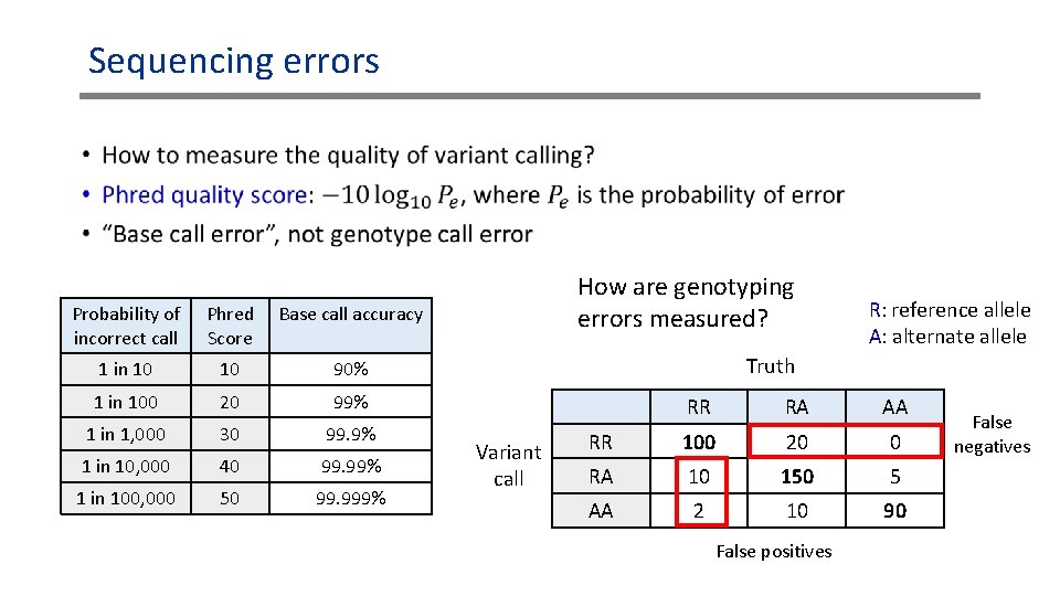
Sequencing errors • Probability of incorrect call How are genotyping errors measured? Phred Base call accuracy Score 1 in 10 10 90% 1 in 100 20 99% 1 in 1, 000 30 99. 9% 1 in 10, 000 40 99. 99% 1 in 100, 000 50 99. 999% R: reference allele A: alternate allele Truth Variant call RR RA AA RR 100 20 0 RA 10 150 5 AA 2 10 90 False positives False negatives

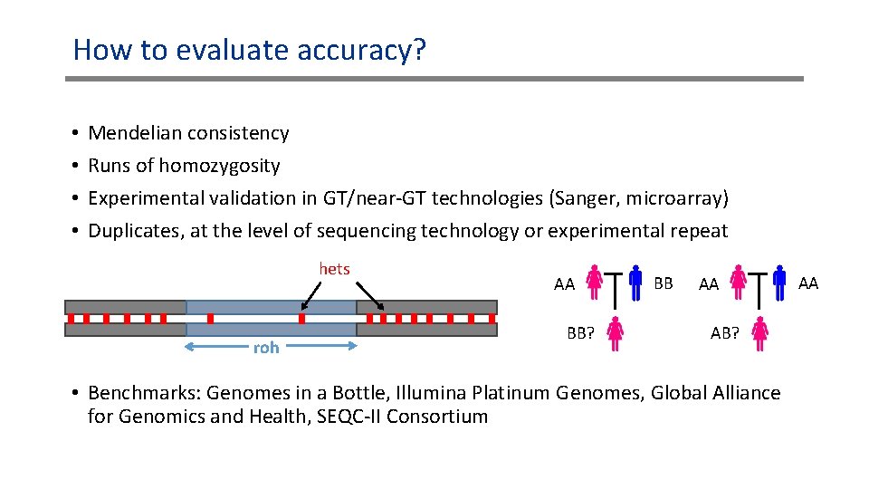
How to evaluate accuracy? • • Mendelian consistency Runs of homozygosity Experimental validation in GT/near-GT technologies (Sanger, microarray) Duplicates, at the level of sequencing technology or experimental repeat hets roh AA BB? BB AA AB? • Benchmarks: Genomes in a Bottle, Illumina Platinum Genomes, Global Alliance for Genomics and Health, SEQC-II Consortium AA

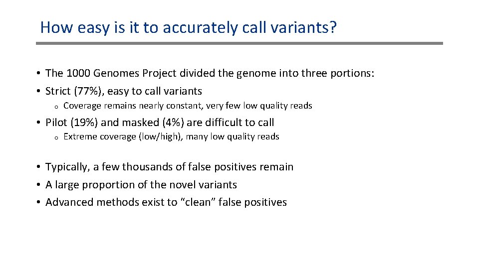
How easy is it to accurately call variants? • The 1000 Genomes Project divided the genome into three portions: • Strict (77%), easy to call variants o Coverage remains nearly constant, very few low quality reads • Pilot (19%) and masked (4%) are difficult to call o Extreme coverage (low/high), many low quality reads • Typically, a few thousands of false positives remain • A large proportion of the novel variants • Advanced methods exist to “clean” false positives

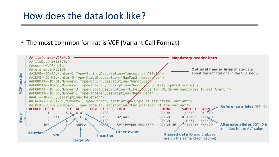
How does the data look like? • The most common format is VCF (Variant Call Format)

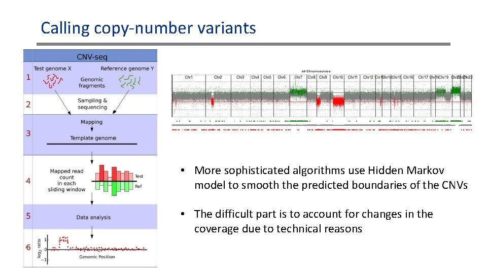
Calling copy-number variants • More sophisticated algorithms use Hidden Markov model to smooth the predicted boundaries of the CNVs • The difficult part is to account for changes in the coverage due to technical reasons

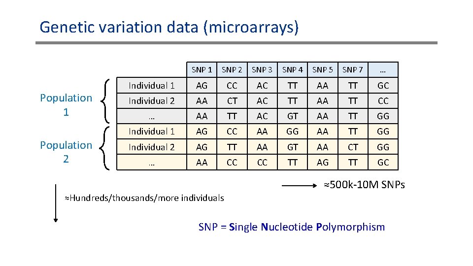
Genetic variation data (microarrays) Population 1 Population 2 SNP 1 SNP 2 SNP 3 SNP 4 SNP 5 SNP 7 … Individual 1 AG CC AC TT AA TT GC Individual 2 AA CT AC TT AA TT CC … AA TT AC GT AA TT GG Individual 1 AG CC AA GG AA TT GG Individual 2 AG TT AA GT AA CT GG … AA CC CC TT AG TT GC ≈500 k-10 M SNPs ≈Hundreds/thousands/more individuals SNP = Single Nucleotide Polymorphism

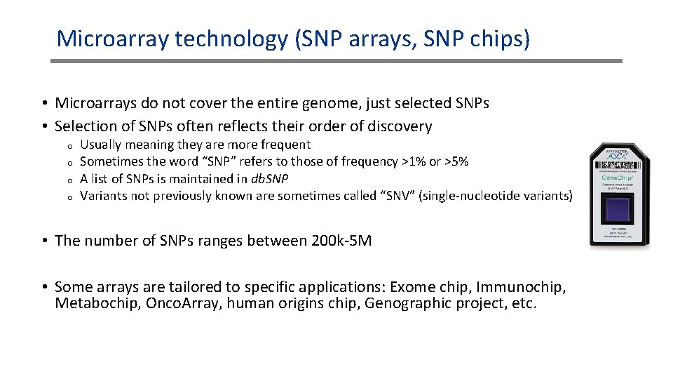
Microarray technology (SNP arrays, SNP chips) • Microarrays do not cover the entire genome, just selected SNPs • Selection of SNPs often reflects their order of discovery o o Usually meaning they are more frequent Sometimes the word “SNP” refers to those of frequency >1% or >5% A list of SNPs is maintained in db. SNP Variants not previously known are sometimes called “SNV” (single-nucleotide variants) • The number of SNPs ranges between 200 k-5 M • Some arrays are tailored to specific applications: Exome chip, Immunochip, Metabochip, Onco. Array, human origins chip, Genographic project, etc.

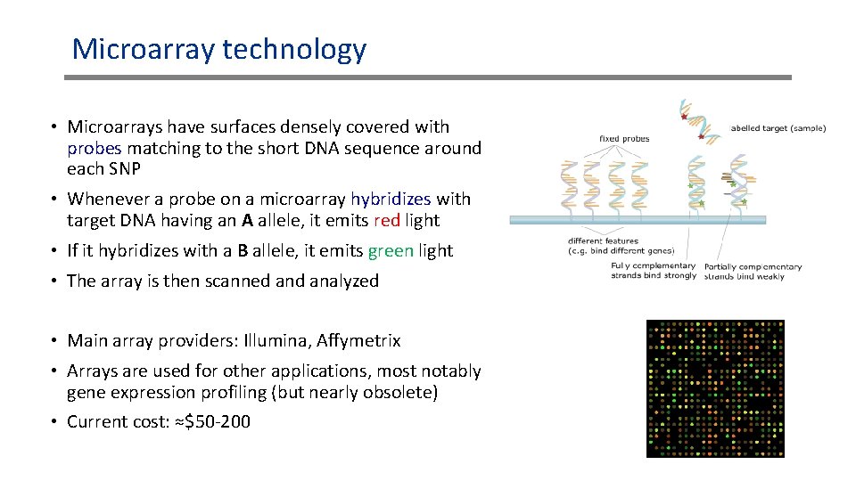
Microarray technology • Microarrays have surfaces densely covered with probes matching to the short DNA sequence around each SNP • Whenever a probe on a microarray hybridizes with target DNA having an A allele, it emits red light • If it hybridizes with a B allele, it emits green light • The array is then scanned analyzed • Main array providers: Illumina, Affymetrix • Arrays are used for other applications, most notably gene expression profiling (but nearly obsolete) • Current cost: ≈$50 -200

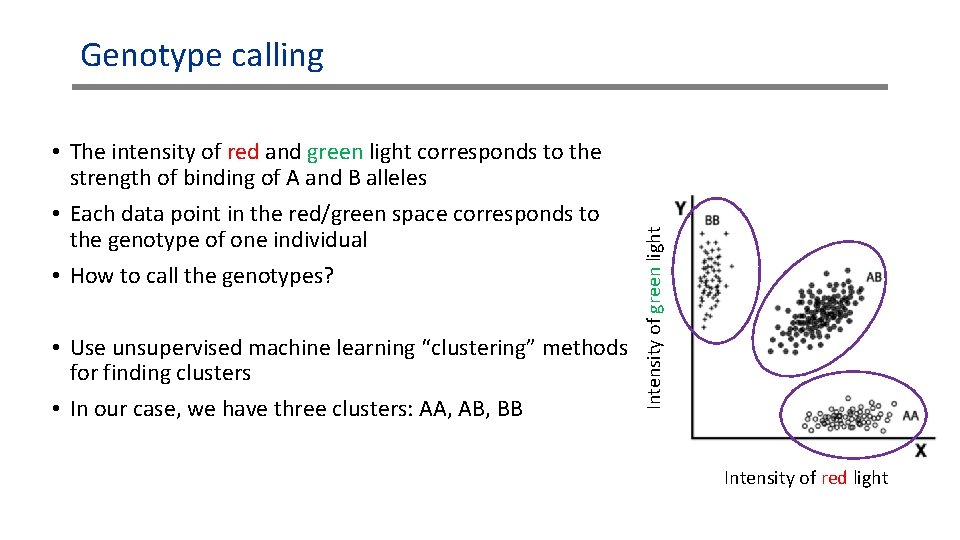
• The intensity of red and green light corresponds to the strength of binding of A and B alleles • Each data point in the red/green space corresponds to the genotype of one individual • How to call the genotypes? • Use unsupervised machine learning “clustering” methods for finding clusters • In our case, we have three clusters: AA, AB, BB Intensity of green light Genotype calling Intensity of red light

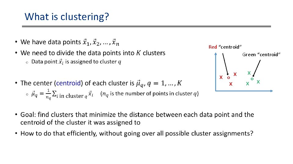
What is clustering? • Red “centroid” Green “centroid” x o x x

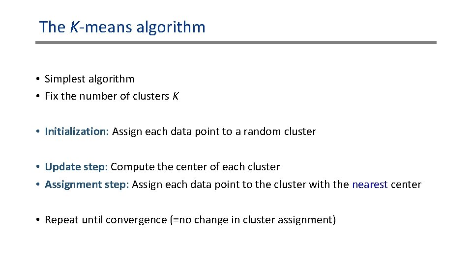
The K-means algorithm • Simplest algorithm • Fix the number of clusters K • Initialization: Assign each data point to a random cluster • Update step: Compute the center of each cluster • Assignment step: Assign each data point to the cluster with the nearest center • Repeat until convergence (=no change in cluster assignment)

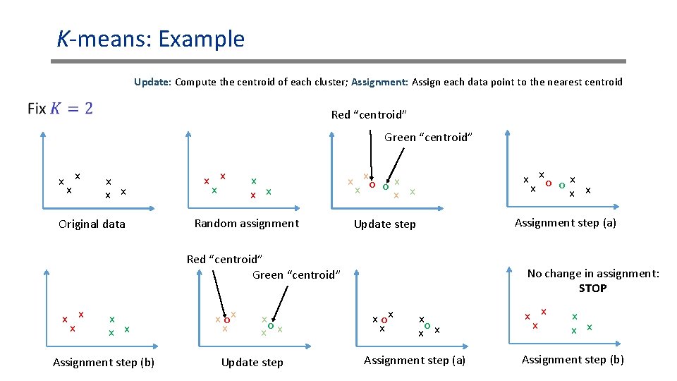
K-means: Example Update: Compute the centroid of each cluster; Assignment: Assign each data point to the nearest centroid Red “centroid” Green “centroid” x x x Original data x x x Random assignment x xo o x x x x Assignment step (a) Update step Red “centroid” Green “centroid” x x x Assignment step (b) x ox x x o x x Update step No change in assignment: STOP x ox x x o x x Assignment step (a) x x x Assignment step (b)

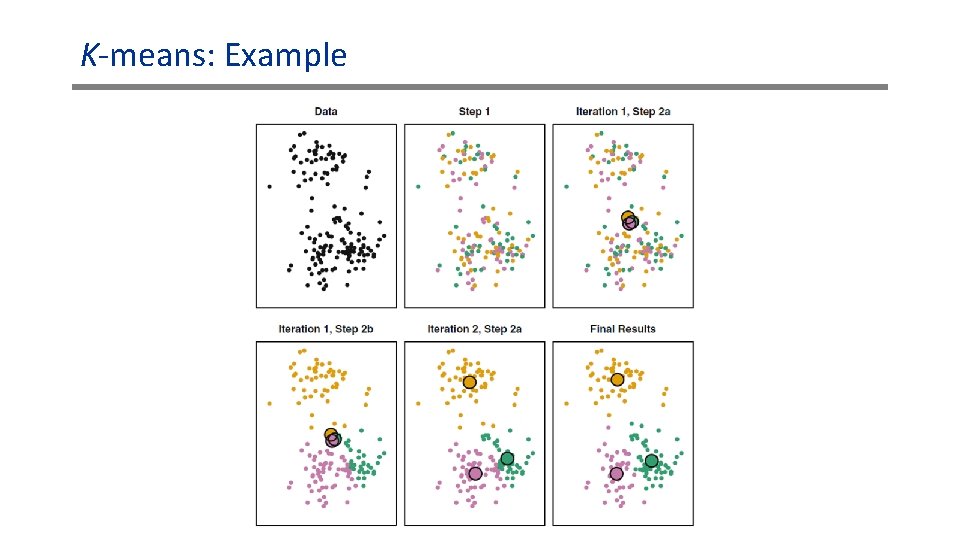
K-means: Example

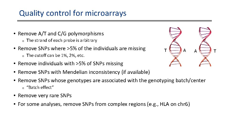
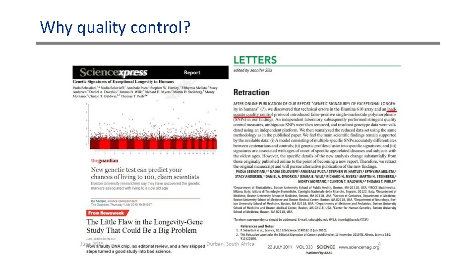
Quality control for microarrays • Remove A/T and C/G polymorphisms o The strand of each probe is arbitrary • Remove SNPs where >5% of the individuals are missing o The cutoff can be 1%, 2%, etc. T A A • Remove individuals with >5% of SNPs missing • Remove SNPs with Mendelian inconsistency (if available) • Remove SNPs whose genotypes are associated with the genotyping batch/center o “Batch effect” • Remove very rare SNPs • For some analyses, remove SNPs from complex regions (e. g. , HLA on chr 6) T

Why quality control?

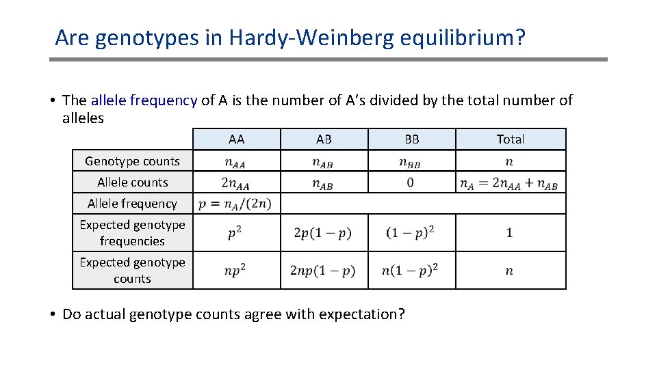
Are genotypes in Hardy-Weinberg equilibrium? • The allele frequency of A is the number of A’s divided by the total number of alleles AA AB BB Genotype counts Allele frequency Expected genotype frequencies Expected genotype counts • Do actual genotype counts agree with expectation? Total

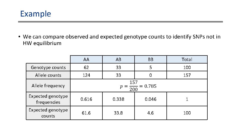
Example • We can compare observed and expected genotype counts to identify SNPs not in HW equilibrium AA AB BB Total Genotype counts 62 33 5 100 Allele counts 124 33 0 157 Expected genotype frequencies 0. 616 0. 338 0. 046 1 Expected genotype counts 61. 6 33. 8 4. 6 100 Allele frequency

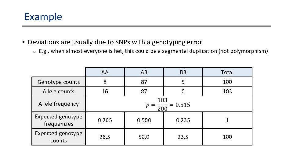
Example • Deviations are usually due to SNPs with a genotyping error o E. g. , when almost everyone is het, this could be a segmental duplication (not polymorphism) AA AB BB Total Genotype counts 8 87 5 100 Allele counts 16 87 0 103 Expected genotype frequencies 0. 265 0. 500 0. 235 1 Expected genotype counts 26. 5 50. 0 23. 5 100 Allele frequency

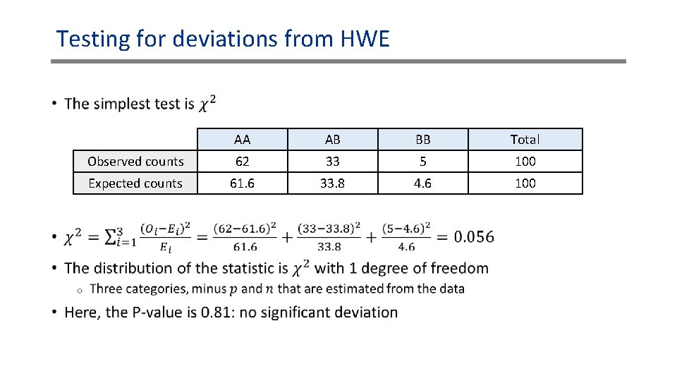
Testing for deviations from HWE • AA AB BB Total Observed counts 62 33 5 100 Expected counts 61. 6 33. 8 4. 6 100

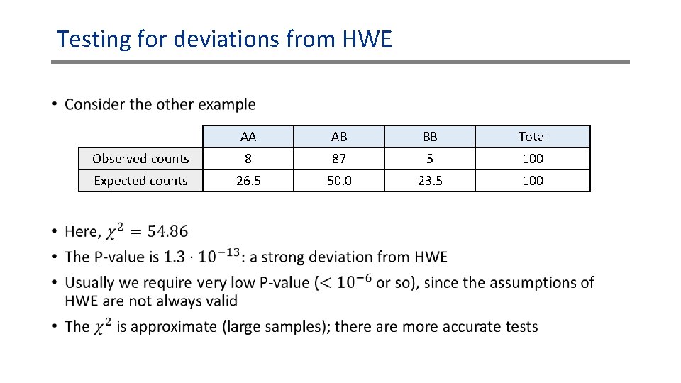
Testing for deviations from HWE • AA AB BB Total Observed counts 8 87 5 100 Expected counts 26. 5 50. 0 23. 5 100

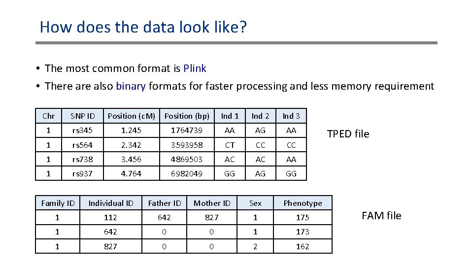
How does the data look like? • The most common format is Plink • There also binary formats for faster processing and less memory requirement Chr SNP ID Position (c. M) Position (bp) Ind 1 Ind 2 Ind 3 1 rs 345 1. 245 1764739 AA AG AA 1 rs 564 2. 342 3593958 CT CC CC 1 rs 738 3. 456 4869503 AC AC AA 1 rs 937 4. 764 6982049 GG AG GG Family ID Individual ID Father ID Mother ID Sex Phenotype 1 112 642 827 1 175 1 642 0 0 1 173 1 827 0 0 2 162 TPED file FAM file