Genetic Algorithms Genetic algorithms imitate natural optimization process

Genetic Algorithms • Genetic algorithms imitate natural optimization process, natural selection in evolution. • Developed by John Holland at the University of Michigan for machine learning in 1975. • Similar algorithms developed in Europe in the 1970 s under the name evolutionary strategies • Main difference has been in the nature of the variables: Discrete vs. continuous • Class is called evolutionary algorithms • Will cover also differential evolution.

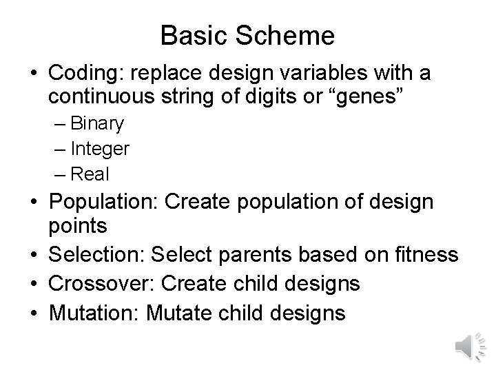
Basic Scheme • Coding: replace design variables with a continuous string of digits or “genes” – Binary – Integer – Real • Population: Create population of design points • Selection: Select parents based on fitness • Crossover: Create child designs • Mutation: Mutate child designs

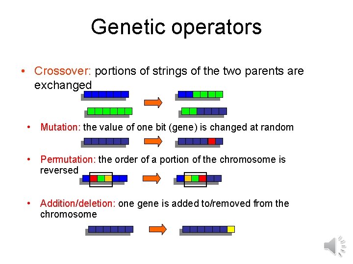
Genetic operators • Crossover: portions of strings of the two parents are exchanged • Mutation: the value of one bit (gene) is changed at random • Permutation: the order of a portion of the chromosome is reversed • Addition/deletion: one gene is added to/removed from the chromosome

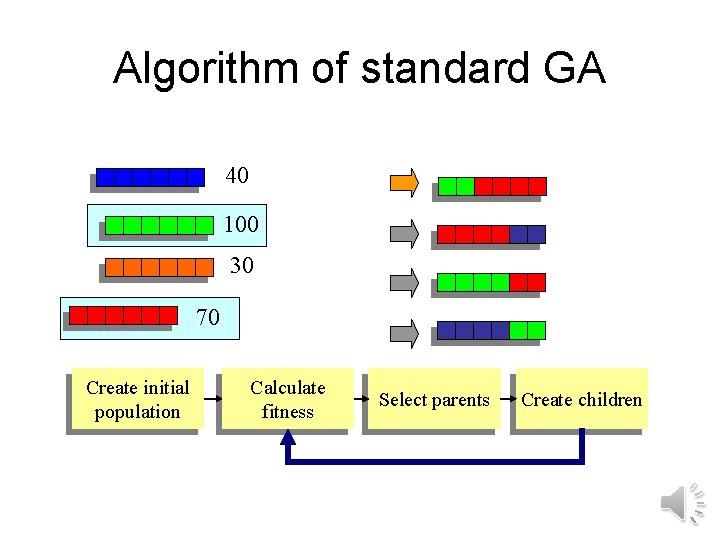
Algorithm of standard GA 40 100 30 70 Create initial population Calculate fitness Select parents Create children

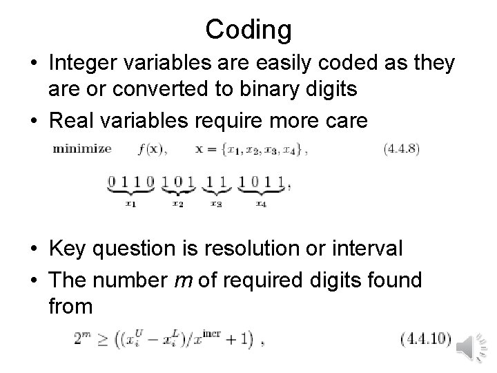
Coding • Integer variables are easily coded as they are or converted to binary digits • Real variables require more care • Key question is resolution or interval • The number m of required digits found from

Stacking sequence optimization • For many practical problems angles limited to 0 -deg, 45 -deg, 90 -deg. • Ply thickness given by manufacturer • Stacking sequence optimization a combinatorial problem • Genetic algorithms effective and easy to implement, but do not deal well with constraints

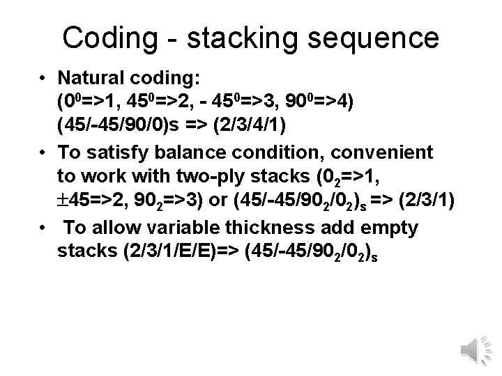
Coding - stacking sequence • Natural coding: (00=>1, 450=>2, - 450=>3, 900=>4) (45/-45/90/0)s => (2/3/4/1) • To satisfy balance condition, convenient to work with two-ply stacks (02=>1, 45=>2, 902=>3) or (45/-45/902/02)s => (2/3/1) • To allow variable thickness add empty stacks (2/3/1/E/E)=> (45/-45/902/02)s

Initial population • Random number generator used • Typical function call is rand(seed) • Seed updated after call to avoid repeating the same number. See Matlab help on how to change seed (state). • Need to transform random numbers to values of alleles.

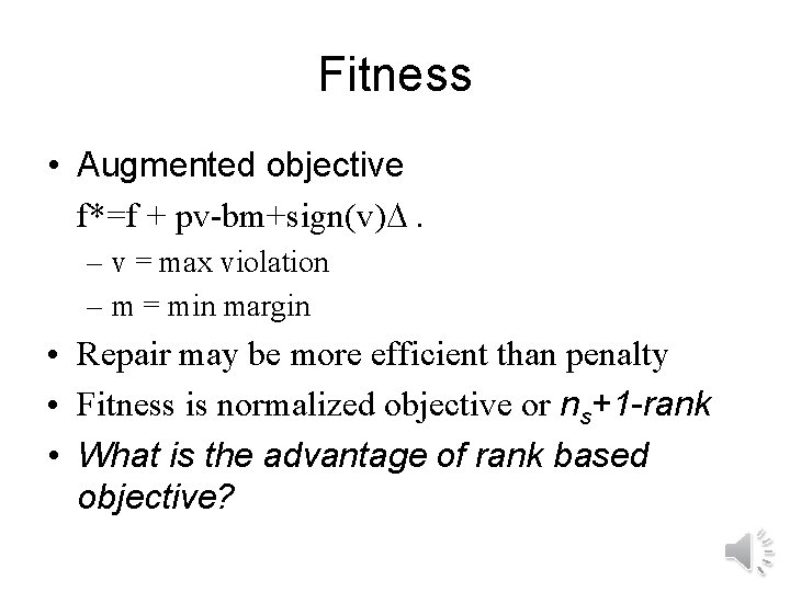
Fitness • Augmented objective f*=f + pv-bm+sign(v) . – v = max violation – m = min margin • Repair may be more efficient than penalty • Fitness is normalized objective or ns+1 -rank • What is the advantage of rank based objective?

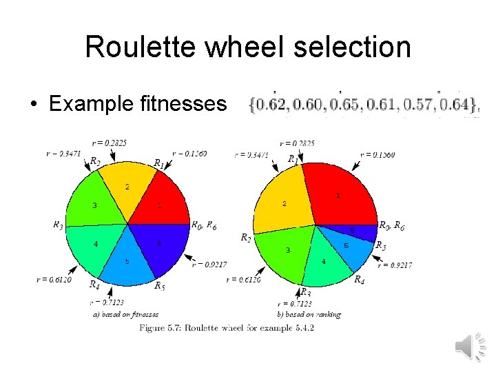
Roulette wheel selection • Example fitnesses

Single Point Crossover • Parent designs [04/± 452/902]s and [± 454/02]s • • Parent 1 [1/1/2/2/ 3] Parent 2 [2/2/ 1] One child [1/1/2/2/1] That is: [04/± 452/02]s

Other kinds of crossover • • • Multiple point crossover Hitchhiking problem Uniform crossover Random crossover for real numbers Multi-parent crossover

Mutation and stack swap • [1/1/2/2/3]=> [1/1/2/3/3] • [04/± 452/902]s => [04/± 45/904]s • [1/1/2/2/3]=> [1/2/3] • [04/± 452/902]s => [(02/± 45)2/902]s

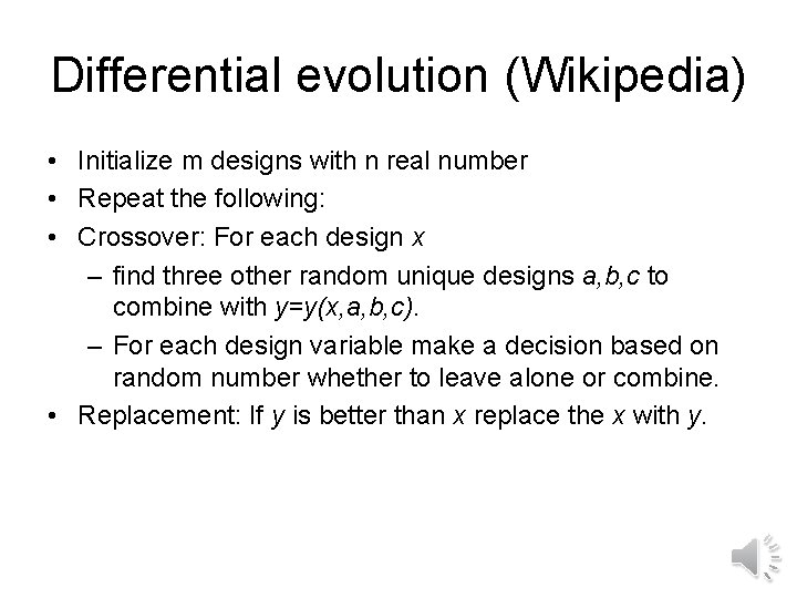
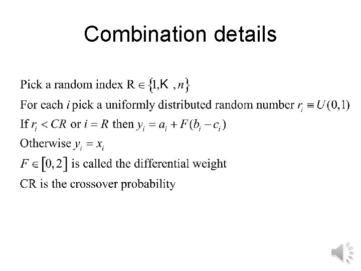
Differential evolution (Wikipedia) • Initialize m designs with n real number • Repeat the following: • Crossover: For each design x – find three other random unique designs a, b, c to combine with y=y(x, a, b, c). – For each design variable make a decision based on random number whether to leave alone or combine. • Replacement: If y is better than x replace the x with y.

Combination details

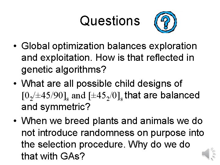
Questions • Global optimization balances exploration and exploitation. How is that reflected in genetic algorithms? • What are all possible child designs of [02/± 45/90]s and [± 452/0]s that are balanced and symmetric? • When we breed plants and animals we do not introduce randomness on purpose into the selection procedure. Why do we do that with GAs?

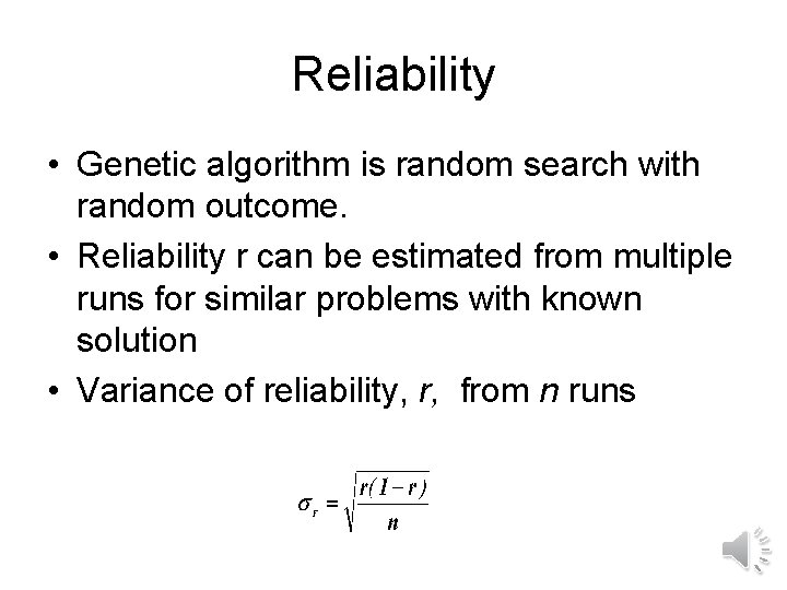
Reliability • Genetic algorithm is random search with random outcome. • Reliability r can be estimated from multiple runs for similar problems with known solution • Variance of reliability, r, from n runs

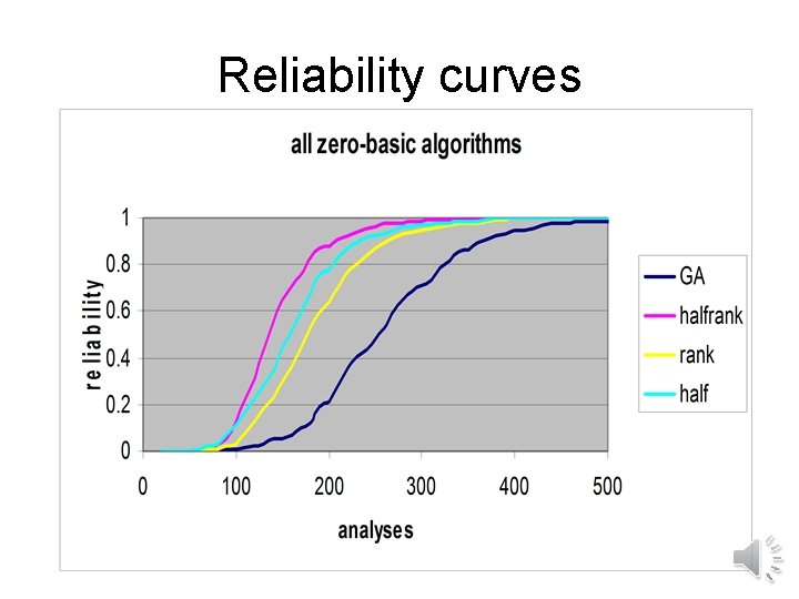
Reliability curves

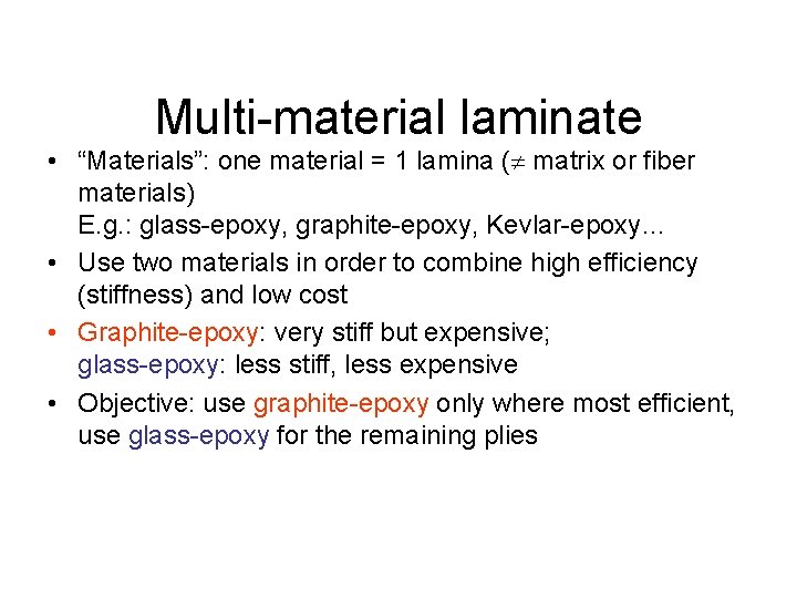
Multi-material laminate • “Materials”: one material = 1 lamina ( matrix or fiber materials) E. g. : glass-epoxy, graphite-epoxy, Kevlar-epoxy… • Use two materials in order to combine high efficiency (stiffness) and low cost • Graphite-epoxy: very stiff but expensive; glass-epoxy: less stiff, less expensive • Objective: use graphite-epoxy only where most efficient, use glass-epoxy for the remaining plies

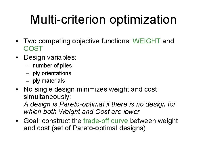
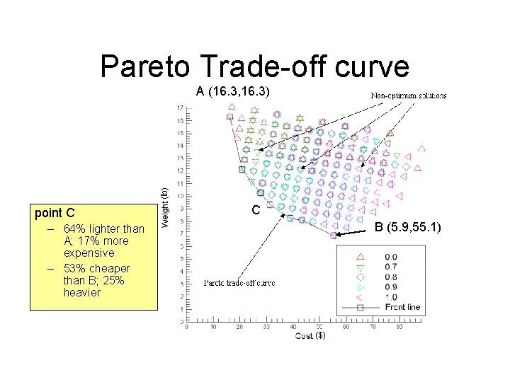
Multi-criterion optimization • Two competing objective functions: WEIGHT and COST • Design variables: – number of plies – ply orientations – ply materials • No single design minimizes weight and cost simultaneously: A design is Pareto-optimal if there is no design for which both Weight and Cost are lower • Goal: construct the trade-off curve between weight and cost (set of Pareto-optimal designs)

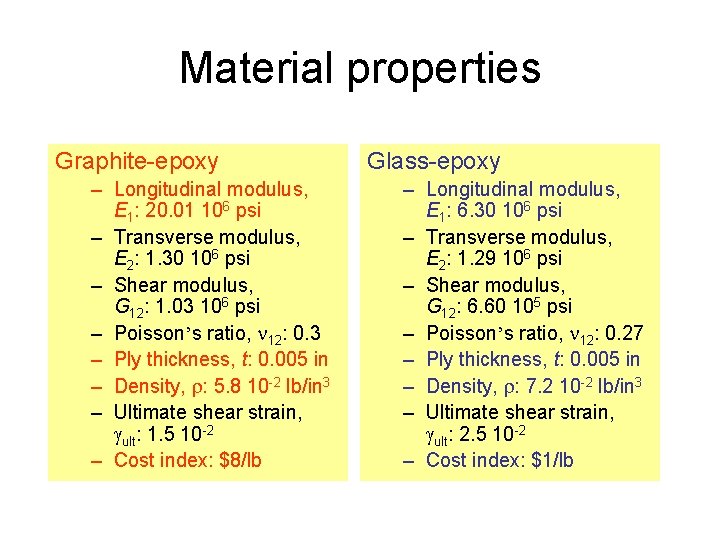
Material properties Graphite-epoxy – Longitudinal modulus, E 1: 20. 01 106 psi – Transverse modulus, E 2: 1. 30 106 psi – Shear modulus, G 12: 1. 03 106 psi – Poisson’s ratio, 12: 0. 3 – Ply thickness, t: 0. 005 in – Density, : 5. 8 10 -2 lb/in 3 – Ultimate shear strain, ult: 1. 5 10 -2 – Cost index: $8/lb Glass-epoxy – Longitudinal modulus, E 1: 6. 30 106 psi – Transverse modulus, E 2: 1. 29 106 psi – Shear modulus, G 12: 6. 60 105 psi – Poisson’s ratio, 12: 0. 27 – Ply thickness, t: 0. 005 in – Density, : 7. 2 10 -2 lb/in 3 – Ultimate shear strain, ult: 2. 5 10 -2 – Cost index: $1/lb

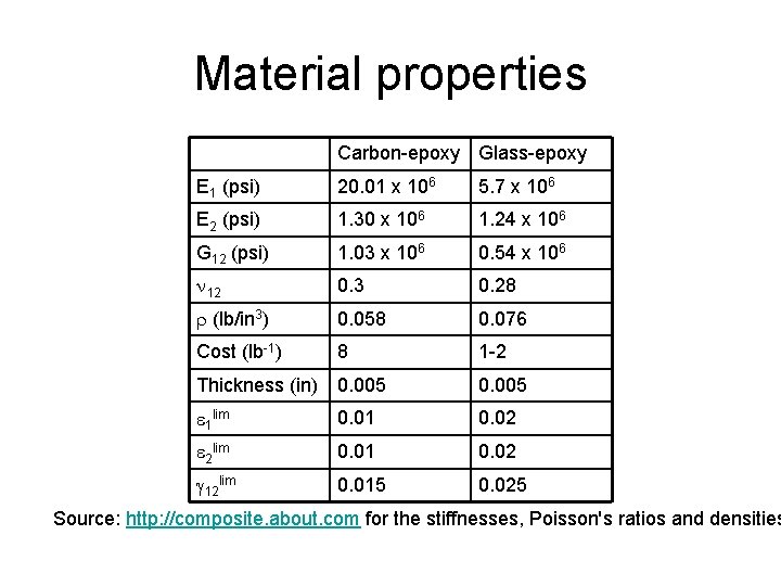
Material properties Carbon-epoxy Glass-epoxy E 1 (psi) 20. 01 x 106 5. 7 x 106 E 2 (psi) 1. 30 x 106 1. 24 x 106 G 12 (psi) 1. 03 x 106 0. 54 x 106 12 0. 3 0. 28 (lb/in 3) 0. 058 0. 076 Cost (lb-1) 8 1 -2 Thickness (in) 0. 005 1 lim 0. 01 0. 02 2 lim 0. 01 0. 02 12 lim 0. 015 0. 025 Source: http: //composite. about. com for the stiffnesses, Poisson's ratios and densities

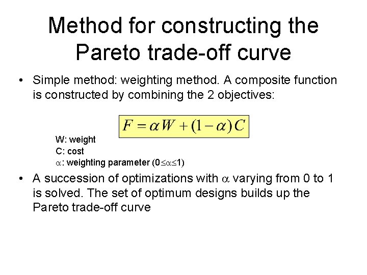
Method for constructing the Pareto trade-off curve • Simple method: weighting method. A composite function is constructed by combining the 2 objectives: W: weight C: cost : weighting parameter (0 1) • A succession of optimizations with varying from 0 to 1 is solved. The set of optimum designs builds up the Pareto trade-off curve

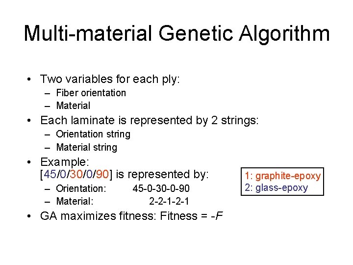
Multi-material Genetic Algorithm • Two variables for each ply: – Fiber orientation – Material • Each laminate is represented by 2 strings: – Orientation string – Material string • Example: [45/0/30/0/90] is represented by: – Orientation: – Material: 45 -0 -30 -0 -90 2 -2 -1 • GA maximizes fitness: Fitness = -F 1: graphite-epoxy 2: glass-epoxy

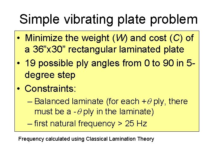
Simple vibrating plate problem • Minimize the weight (W) and cost (C) of a 36”x 30” rectangular laminated plate • 19 possible ply angles from 0 to 90 in 5 degree step • Constraints: – Balanced laminate (for each + ply, there must be a - ply in the laminate) – first natural frequency > 25 Hz Frequency calculated using Classical Lamination Theory

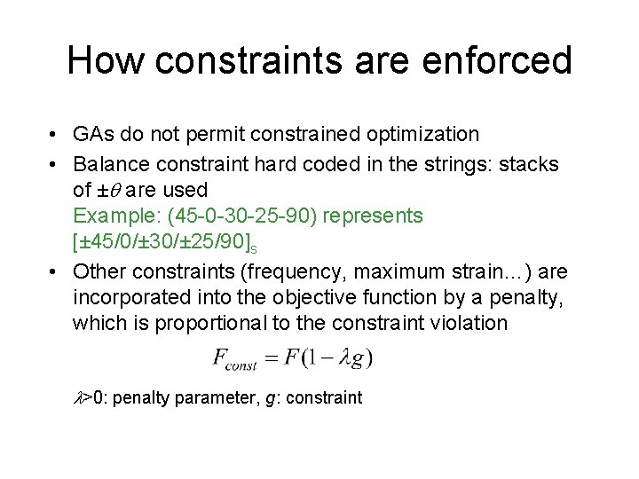
How constraints are enforced • GAs do not permit constrained optimization • Balance constraint hard coded in the strings: stacks of ± are used Example: (45 -0 -30 -25 -90) represents [± 45/0/± 30/± 25/90]s • Other constraints (frequency, maximum strain…) are incorporated into the objective function by a penalty, which is proportional to the constraint violation >0: penalty parameter, g: constraint

Pareto Trade-off curve (lb) A (16. 3, 16. 3) point C C B (5. 9, 55. 1) – 64% lighter than A; 17% more expensive – 53% cheaper than B; 25% heavier ($)

Optimum laminates • Cost minimization: [± 5010/0]s, cost = 16. 33, weight = 16. 33 • Weight minimization: [± 505/0]s, cost = 55. 12, weight = 6. 89 • Intermediate design: [± 502/± 505]s, cost = 27. 82, weight = 10. 28 Intermediate optimum laminates: sandwich-type laminates Midplane Graphite-epoxy as outer plies for a high frequency Glass-epoxy in the core layers to increase thickness