Introduction to Genetic Algorithms Genetic Algorithms Weve covered

Introduction to Genetic Algorithms

Genetic Algorithms • We’ve covered enough material that we can write programs that use genetic algorithms! – More advanced example of using arrays – Could be better written in most cases using objects

Evolution in Computers • Genetic Algorithms – most widely known work by John Holland • Based on Darwinian Evolution – In a competitive environment, strongest, “most fit” of a species survive, weak die – Survivors pass their good genes on to offspring – Occasional mutation

Evolution in Computers • Same idea as Darwinian Evolution – Population of computer program / solution treated like biological organisms in a competitive environment • Computer programs / solutions typically encoded as a bit string – Survival Instinct – have computer programs compete with one another in some environment, evolve with mutation and sexual recombination

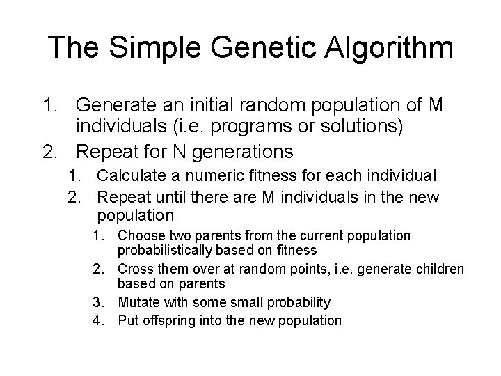
The Simple Genetic Algorithm 1. Generate an initial random population of M individuals (i. e. programs or solutions) 2. Repeat for N generations 1. Calculate a numeric fitness for each individual 2. Repeat until there are M individuals in the new population 1. Choose two parents from the current population probabilistically based on fitness 2. Cross them over at random points, i. e. generate children based on parents 3. Mutate with some small probability 4. Put offspring into the new population

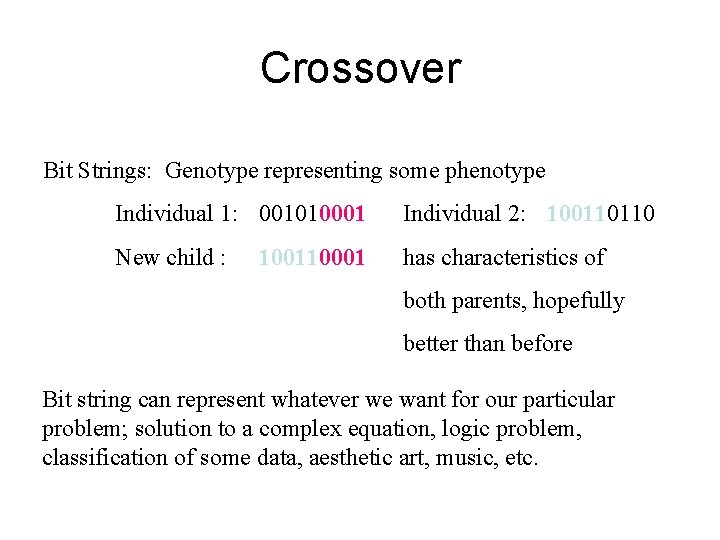
Crossover Bit Strings: Genotype representing some phenotype Individual 1: 001010001 Individual 2: 100110110 New child : has characteristics of 100110001 both parents, hopefully better than before Bit string can represent whatever we want for our particular problem; solution to a complex equation, logic problem, classification of some data, aesthetic art, music, etc.

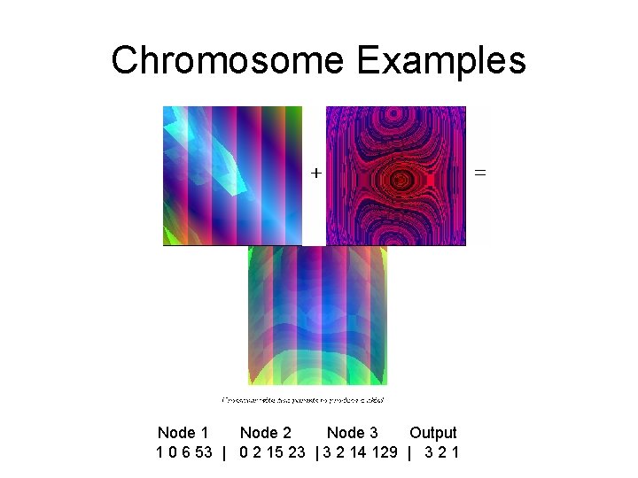
Chromosome Examples Node 1 Node 2 Node 3 Output 1 0 6 53 | 0 2 15 23 | 3 2 14 129 | 3 2 1

Chromosome Examples Gen 3 : A=FF[F[A+F[-FF-AFF]]]F Gen 5 : A=FF[F[A+F[-FF-FFA[-]]]] Gen 7 : A= FF[F-[F[A+F[-[A][]]]][A+F[-F-A[]]]]F

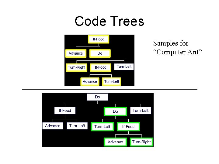
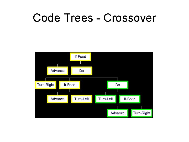
Code Trees Samples for “Computer Ant”

Code Trees - Crossover

Program Example • The Traveling Salesman Problem (TSP) – Member of a class of problems called NPComplete • Hard problems with no known polynomial time solution, only exponential time • Other NP problems map to a NP-Complete problem in polynomial time, suggesting these are the hardest problems in the class • NP-Complete problems are good candidates for applying genetic algorithms and approximation techniques – Problem space too large to solve exhaustively – Generally not guaranteed to solve the problem optimally

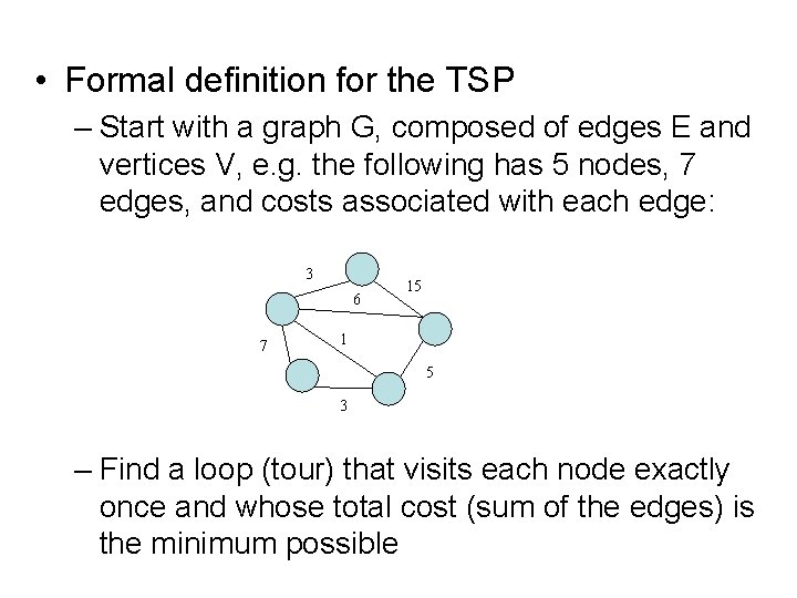
• Formal definition for the TSP – Start with a graph G, composed of edges E and vertices V, e. g. the following has 5 nodes, 7 edges, and costs associated with each edge: 3 6 7 15 1 5 3 – Find a loop (tour) that visits each node exactly once and whose total cost (sum of the edges) is the minimum possible

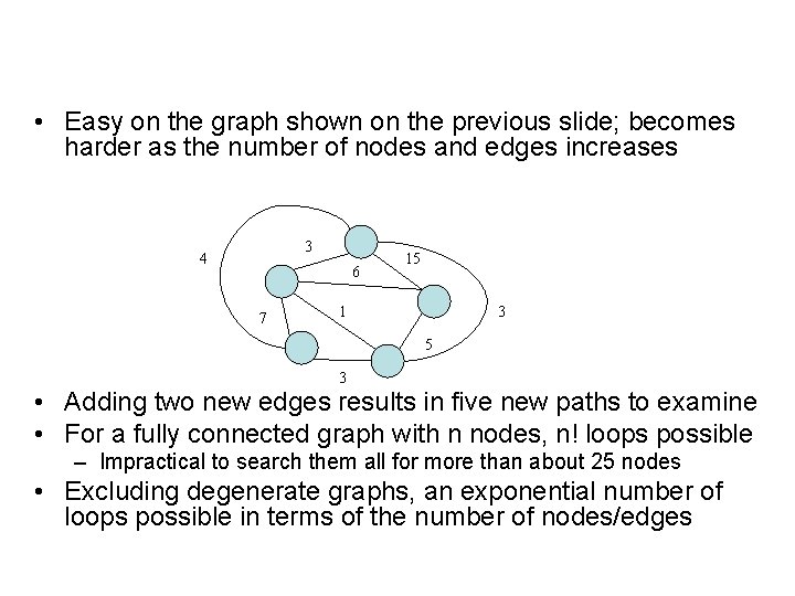
• Easy on the graph shown on the previous slide; becomes harder as the number of nodes and edges increases 3 4 6 7 15 1 3 5 3 • Adding two new edges results in five new paths to examine • For a fully connected graph with n nodes, n! loops possible – Impractical to search them all for more than about 25 nodes • Excluding degenerate graphs, an exponential number of loops possible in terms of the number of nodes/edges

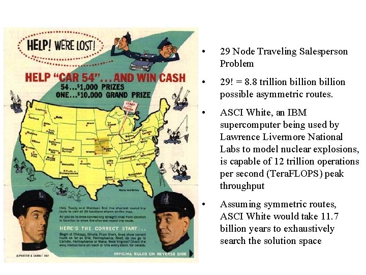
• 29 Node Traveling Salesperson Problem • 29! = 8. 8 trillion billion possible asymmetric routes. • ASCI White, an IBM supercomputer being used by Lawrence Livermore National Labs to model nuclear explosions, is capable of 12 trillion operations per second (Tera. FLOPS) peak throughput • Assuming symmetric routes, ASCI White would take 11. 7 billion years to exhaustively search the solution space

• Genetic algorithms approximation for a solution – Randomly generate a population of agents • Each agent represents an entire solution, i. e. a random ordering of each node representing a loop – Given nodes 1 -6, we might generate 423651 to represent the loop of visiting 4 first, then 2, then 3, then 6, then 5, then 1, then back to 4 – Assign each agent a fitness value • Fitness is just the sum of the edges in the loop; lower is more fit – Evolve a new, hopefully better, generation of the same number of agents • Select two parents randomly, but higher probability of selection if better fitness • New generation formed by crossover and mutation

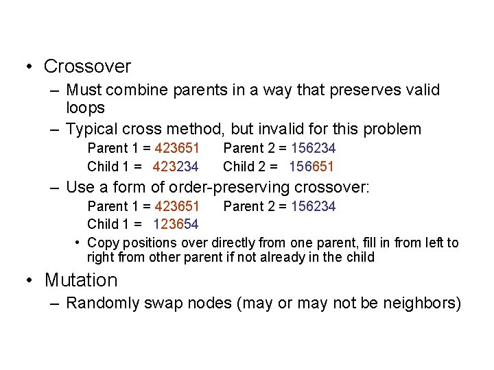
• Crossover – Must combine parents in a way that preserves valid loops – Typical cross method, but invalid for this problem Parent 1 = 423651 Child 1 = 423234 Parent 2 = 156234 Child 2 = 156651 – Use a form of order-preserving crossover: Parent 1 = 423651 Parent 2 = 156234 Child 1 = 123654 • Copy positions over directly from one parent, fill in from left to right from other parent if not already in the child • Mutation – Randomly swap nodes (may or may not be neighbors)

• Run the program! • Describe major components of the code • If you’re interested in more about genetic algorithms, there is a ton of information if you google “genetic algorithms”

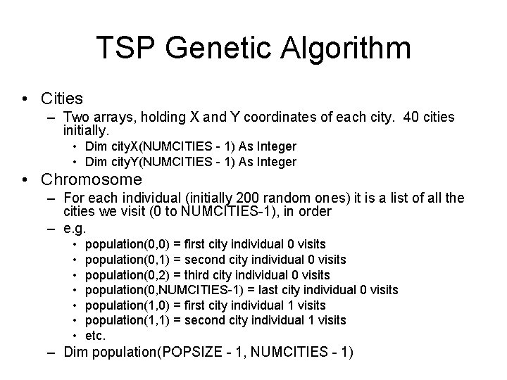
TSP Genetic Algorithm • Cities – Two arrays, holding X and Y coordinates of each city. 40 cities initially. • Dim city. X(NUMCITIES - 1) As Integer • Dim city. Y(NUMCITIES - 1) As Integer • Chromosome – For each individual (initially 200 random ones) it is a list of all the cities we visit (0 to NUMCITIES-1), in order – e. g. • • population(0, 0) = first city individual 0 visits population(0, 1) = second city individual 0 visits population(0, 2) = third city individual 0 visits population(0, NUMCITIES-1) = last city individual 0 visits population(1, 0) = first city individual 1 visits population(1, 1) = second city individual 1 visits etc. – Dim population(POPSIZE - 1, NUMCITIES - 1)

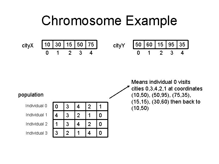
Chromosome Example city. X 10 30 15 50 75 0 1 2 3 4 city. Y population Individual 0 0 3 4 2 1 Individual 1 4 3 2 1 0 Individual 2 1 3 4 2 0 Individual 3 3 2 1 4 0 50 60 15 95 35 0 1 2 3 4 Means individual 0 visits cities 0, 3, 4, 2, 1 at coordinates (10, 50), (50, 95), (75, 35), (15, 15), (30, 60) then back to (10, 50)

TSP Genetic Algorithm • Uses crossover and mutation described on previous slide • Fitness is distance for each individual • Hard-coded to run 1000 generations, display the individual that has the shortest path each generation