GeneralizedLinearModels LinearModel u response variable intercept slope explanatory

Generalized Linear Models • Linear Model u response variable ~ intercept + slope * explanatory variable u lm(y~ x + f ・・・),lm(y~x + f -1) (no intercept) u. Generalized Linear Model u Model &Link function ~ intercept + slope * explanatory variable u glm(y ~ x, data = d, family = poisson)
 (discrete) (continuous) Probability Random numbers generation")
Other Generalized Linear Models (chap 6 p 114) (discrete) (continuous) Probability Random numbers generation Family in glm() Standard link function Binomial rbinom() binomial logit Poisson rpois() poisson log Negative Binomial rnbinom() (glb. nb() function) log Gamma rgamma() gamma log, inverse Normal rnorm() gaussian identity
")
Generalized Linear Models u. Generalized Linear Model glm(y ~ x, data = d, family = poisson) u. Family (Modelled Probability Distribution) ubinomial(link = “logit“) 2項分布(規定試行中の発生数) ugaussian(link = “identity”) 正規分布 u. Gamma(link = “inverse”) ガンマ分布(正のみ) uinverse. gaussian(link = “ 1/mu^2”) 逆ガウス分布 upoisson(link = “log”) ポアソン分布(一定時間中の発生回数) uquasi(link = “identity”, variance = “constant”)正規分布(不均一) u quasibinomial(link = “logit”) 2項分布(分散不均一) u quasipoisson(link = “log”) ポアソン分布(分散不均一)
 Likelihood • 確率分布の形とパラメータの値θが決まれば,確率変数Xにつ いて値xが得られる確率(確率密度)が計算できる. • For given Probability Distribution and relevant parameter")
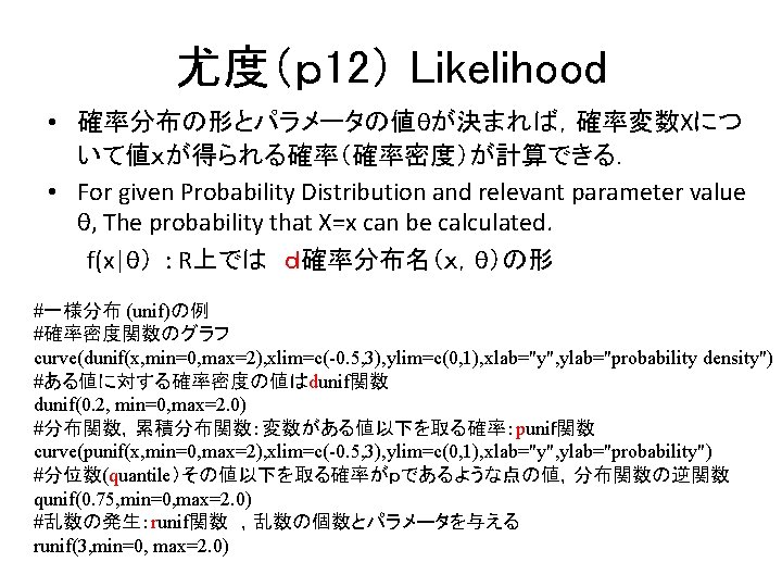
尤度(p 12) Likelihood • 確率分布の形とパラメータの値θが決まれば,確率変数Xにつ いて値xが得られる確率(確率密度)が計算できる. • For given Probability Distribution and relevant parameter value θ, The probability that X=x can be calculated. f(x|θ) : R上では d確率分布名(x,θ)の形 • 逆に,データX=xが与えられたとき,値xが得られる確率をパラ メータの値θの関数と考え尤度 (likelihood)という. • Conversely, For given Probability Distribution and realized observations X=x, the probability can be considered as a function of parameter θ. That function is called as likelihood function. f(θ|x)

二項分布の例と尤度関数 Binomial Distribution of Bernoulli trial • つぼのなかに赤球r個,白球w個あり,1つ取り出して色を記録 して戻すことをn回繰り返す。 Get one ball out from the bottle, including r Red balls and w White balls. Repeat n trials. • 赤の回数Yがyを取る確率は母数φ=r/(r+w)の関数となる。 The probability of Y (number of Red balls out of n balls) is given as Binomial function with single parameter φ=r/(r+w). • 実際に赤が8回,白が2回でた場合には,そのことが起こる確率 を母数φの関数と見なしたものを尤度関数L(φ)と呼ぶ. When 8 red and 2 white balls appeared, the probability is considered as a function of unknown parameter φ. That is Likelihood function.
, ylab=\"probability\",")
二項分布の例と尤度関数 Likelihood function of Bernoulli Trial #二項分布の関数形Binomial function:Rではdbinom barplot(dbinom(0: 10, size=10, prob=0. 6), ylab="probability", space=0 , names=as. character(0: 10), col="white") #赤が8回,白が2回でた場合の尤度関数 L(φ) # Likelihood function for 8 red and 2 white balls. Lik <- function(phi) {dbinom(8, size=10, phi)} curve(Lik(x), 0, 1) #尤度関数の対数値を対数尤度関数(Log. Likelihood) # Logarithm of likelihood function LLik <- function(phi) {log(dbinom(8, size=10, phi))} curve(LLik(x), 0. 05, 0. 95)
 Maximum log. Likelihood • 赤が8回,白が2回でた場合の尤度関数, 対数尤度関数 Loglikelihood これを母数φで微分すると,Differentiate by parameter φ 最大値は最後の分子が0になる, φ=8/10=")
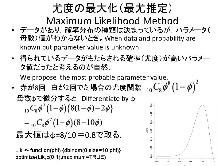
尤度の最大化(最尤推定) Maximum log. Likelihood • 赤が8回,白が2回でた場合の尤度関数, 対数尤度関数 Loglikelihood これを母数φで微分すると,Differentiate by parameter φ 最大値は最後の分子が0になる, φ=8/10= 0. 8で取る. Maximum point is φ=8/10= 0. 8. LLik <- function(phi) {log(dbinom(8, size=10, phi))} optimize(LLik, c(0. 01, 0. 99), maximum=TRUE)
 Score Function • 尤度関数をパラメータで偏微分したもの: スコア関数 Score Function: Partial derivative function of the Likelihood.")
スコア関数(尤度の微分) Score Function • 尤度関数をパラメータで偏微分したもの: スコア関数 Score Function: Partial derivative function of the Likelihood. • 最尤推定値はスコア関数= 0の解.パラメータが複数あると きは各パラメータに対するスコア関数= 0の連立方程式の解 Maximum likelihood parameter value is given as the solution of score function = 0. #スコア関数の定義 Scor <- function(phi){phi^7*(1 -phi)*(8 -10*phi)} #スコア関数のグラフ curve(Scor(x), 0, 1) abline(h=0. 0) #スコア関数の= 0の数値解 uniroot(Scor, c(0. 05, 0. 95))

In Applications Parameter value should be explained further as a function of explanatory variables and factors. • Success Rate of Yuzuru Hanyu’s Jumps in a figure skating play. • Success Rate may be related with Temperature of Ice, Elevation of the Ice Link, Time of play, Order of Play, …. • At least The success rate should sit between 0 and 1. • Let us use logit link function.
 Three test methods •")
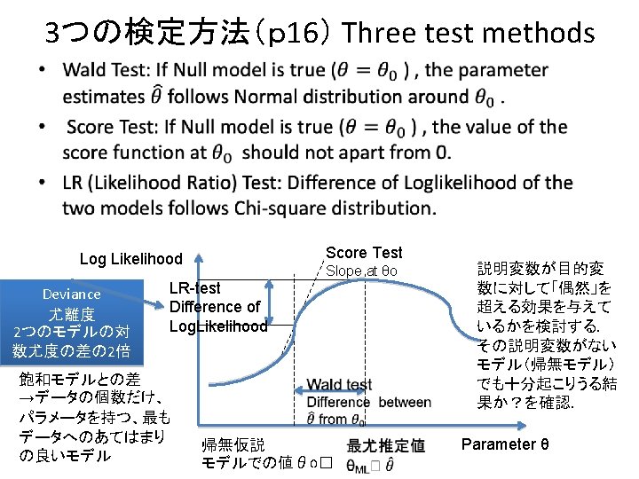
3つの検定方法(p 16) Three test methods •
 Three test methods •")
3つの検定方法(p 16) Three test methods •
 (counting data of occurrence) u. Poisson Model for number of seeds")
Poisson Model (p 49) (counting data of occurrence) u. Poisson Model for number of seeds of a plant, regressed on plant size and nutrification (p 49) u. Maximize log-likelihood glm(y ~ x + f, data = d, family = poisson) #page 19 x 1 <- c(6. 5, 3. 8, 3. 4, 2. 4, 3. 0, 5. 5, 2. 4, 6. 6) x 2 <- c(3. 7, 4. 9, 1. 0, 1. 8, 4. 6, 4. 8, 3. 8, 2. 7) y 1 <- c(8, 5, 2, 0, 1, 11, 4, 9) fit <- glm(y 1~x 1+x 2, family=poisson) summary(fit) #説明変数の係数と切片 coef(fit) #目的変数値と,線形予測子の値 predict(fit, type="response") predict(fit, type="link") #説明変数値が異なる値の場合の予測値 predict(fit, newdata=data_new 1, type="link")
 #page 19 #残差 x 1 <- c(6. 5, 3. 8, 3. 4,")
推定結果の利用(p 23) #page 19 #残差 x 1 <- c(6. 5, 3. 8, 3. 4, 2. 4, 3. 0, 5. 5, 2. 4, 6. 6) #目的変数観測値の残差 x 2 <- c(3. 7, 4. 9, 1. 0, 1. 8, 4. 6, 4. 8, 3. 8, 2. 7) residuals(fit, type="response") y 1 <- c(8, 5, 2, 0, 1, 11, 4, 9) #デビアンス誤差:デビアンスの平方根 fit <- glm(y 1~x 1+x 2, family=poisson) residuals(fit, type="deviance") summary(fit) #ピアソン誤差:残差/分散の平方根 #説明変数の係数と切片 residuals(fit, type="pearson") coef(fit) #目的変数値と,線形予測子の値 predict(fit, type=“response”) predict(fit, type=“link”) #説明変数値が異なる値の場合の予測値 predict(fit, newdata=data_new 1, type=“link”)
 #Wald検定: summaryで表示される summary(fit) #尤度比検定:anovaを呼び出す anova(fit, test=\"Chisq\") anova(fit, test=\"LRT\") #スコア検定:anovaを呼び出す anova(fit, test=\"Rao\") #AICの値")
検定(p 26) #Wald検定: summaryで表示される summary(fit) #尤度比検定:anovaを呼び出す anova(fit, test="Chisq") anova(fit, test="LRT") #スコア検定:anovaを呼び出す anova(fit, test="Rao") #AICの値 AIC(fit) extract. AIC (fit)
- Slides: 19