Gaussian process emulation of multiple outputs Tony OHagan

Gaussian process emulation of multiple outputs Tony O’Hagan, MUCM, Sheffield

Outline � Gaussian process emulators Simulators and emulators � GP modelling � � Multiple outputs Covariance functions � Independent emulators � Transformations to independence � Convolution � Outputs as extra dimension(s) � The multi-output (separable) emulator � The dynamic emulator � � Which � works best? An example

Simulators and emulators �A simulator is a model of a real process � Typically implemented as a computer code � Think of it as a function taking inputs x and giving outputs y � y = f(x) � An emulator is a statistical representation of the function � Expressing knowledge/beliefs about what the output will be at any given input(s) � Built using prior information and a training set of model runs � The GP emulator expresses f as a GP � Conditional on hyperparameters

GP modelling � Mean function � Regression form h(x)Tβ � Used to model broad shape of response � Analogous to universal kriging � Covariance function � Stationary � Often use the Gaussian form σ2 exp{-(x-x′) TD-2(x-x′)} � D is diagonal with correlation lengths on diagonal � Hyperparameters � Uninformative β, σ2 and D priors

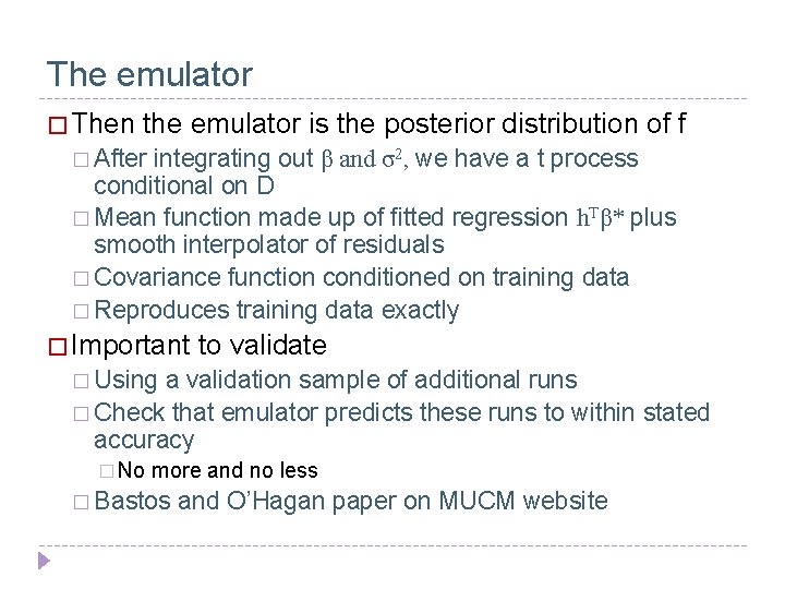
The emulator � Then the emulator is the posterior distribution of f � After integrating out β and σ2, we have a t process conditional on D � Mean function made up of fitted regression h. Tβ* plus smooth interpolator of residuals � Covariance function conditioned on training data � Reproduces training data exactly � Important to validate � Using a validation sample of additional runs � Check that emulator predicts these runs to within stated accuracy � No more and no less � Bastos and O’Hagan paper on MUCM website

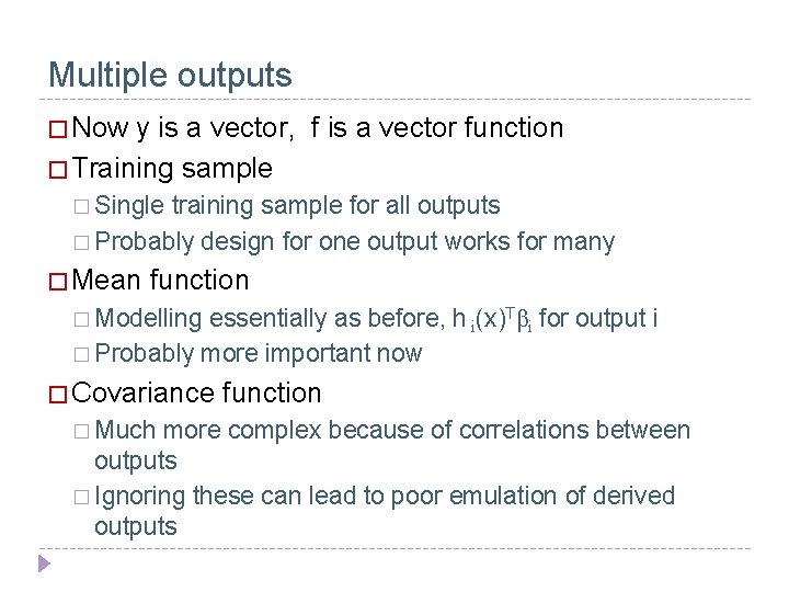
Multiple outputs � Now y is a vector, f is a vector function � Training sample � Single training sample for all outputs � Probably design for one output works for many � Mean function � Modelling essentially as before, h i(x)Tβi for output i � Probably more important now � Covariance � Much function more complex because of correlations between outputs � Ignoring these can lead to poor emulation of derived outputs

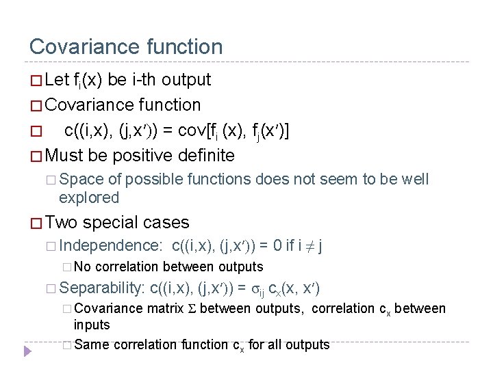
Covariance function � Let fi(x) be i-th output � Covariance function � c((i, x), (j, x′)) = cov[fi (x), fj(x′)] � Must be positive definite � Space of possible functions does not seem to be well explored � Two special cases � Independence: � No c((i, x), (j, x′)) = 0 if i ≠ j correlation between outputs � Separability: � Covariance c((i, x), (j, x′)) = σij cx(x, x′) matrix Σ between outputs, correlation cx between inputs � Same correlation function cx for all outputs

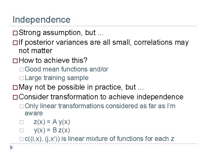
Independence � Strong assumption, but. . . � If posterior variances are all small, correlations may not matter � How to achieve this? � Good mean functions and/or � Large training sample � May not be possible in practice, but. . . � Consider transformation to achieve independence � Only linear transformations considered as far as I’m aware � z(x) = A y(x) � y(x) = B z(x) � c((i, x), (j, x′)) is linear mixture of functions for each z

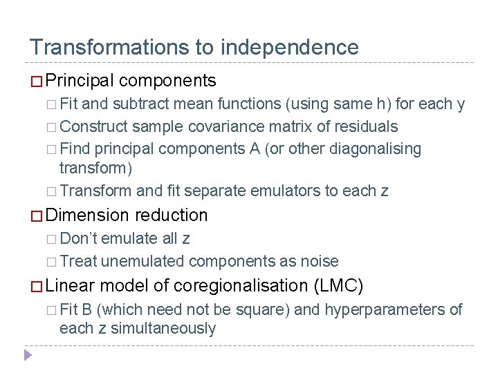
Transformations to independence � Principal components � Fit and subtract mean functions (using same h) for each y � Construct sample covariance matrix of residuals � Find principal components A (or other diagonalising transform) � Transform and fit separate emulators to each z � Dimension reduction � Don’t emulate all z � Treat unemulated components as noise � Linear � Fit model of coregionalisation (LMC) B (which need not be square) and hyperparameters of each z simultaneously

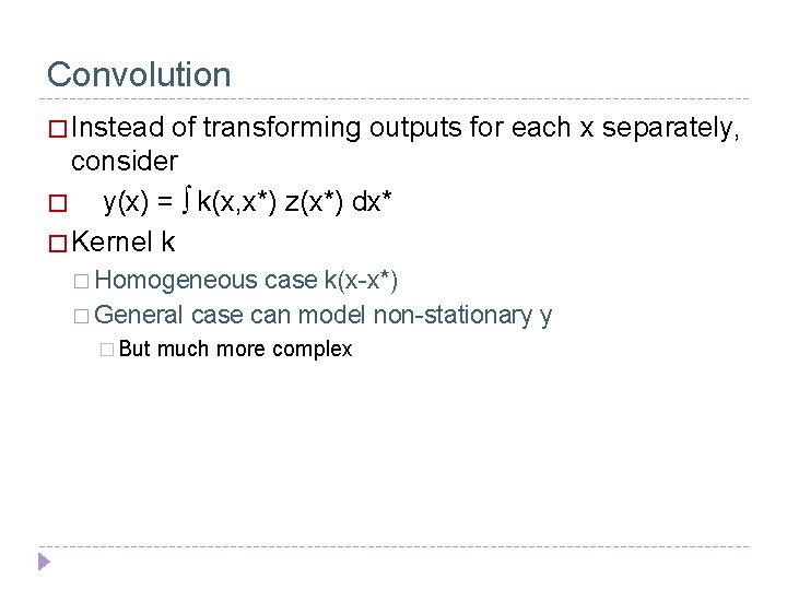
Convolution � Instead of transforming outputs for each x separately, consider � y(x) = ∫ k(x, x*) z(x*) dx* � Kernel k � Homogeneous case k(x-x*) � General case can model non-stationary y � But much more complex

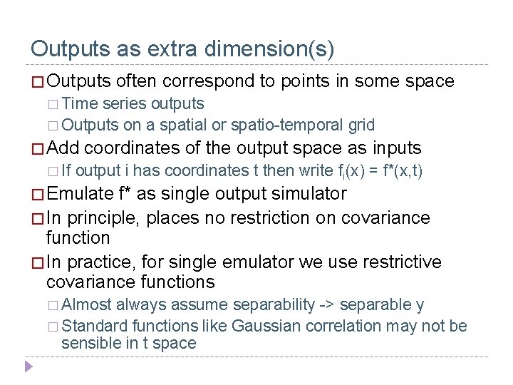
Outputs as extra dimension(s) � Outputs often correspond to points in some space � Time series outputs � Outputs on a spatial or spatio-temporal grid � Add � If coordinates of the output space as inputs output i has coordinates t then write fi(x) = f*(x, t) � Emulate f* as single output simulator � In principle, places no restriction on covariance function � In practice, for single emulator we use restrictive covariance functions � Almost always assume separability -> separable y � Standard functions like Gaussian correlation may not be sensible in t space

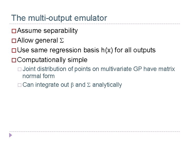
The multi-output emulator � Assume separability � Allow general Σ � Use same regression basis h(x) for all outputs � Computationally simple � Joint distribution of points on multivariate GP have matrix normal form � Can integrate out β and Σ analytically

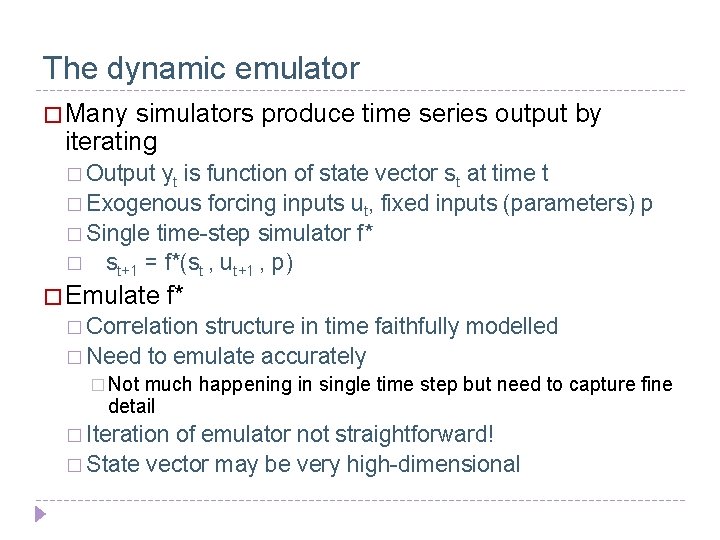
The dynamic emulator � Many simulators produce time series output by iterating � Output yt is � Exogenous function of state vector st at time t forcing inputs ut, fixed inputs (parameters) p � Single time-step simulator f* � st+1 = f*(st , ut+1 , p) � Emulate f* � Correlation structure in time faithfully modelled � Need to emulate accurately � Not much happening in single time step but need to capture fine detail � Iteration of emulator not straightforward! � State vector may be very high-dimensional

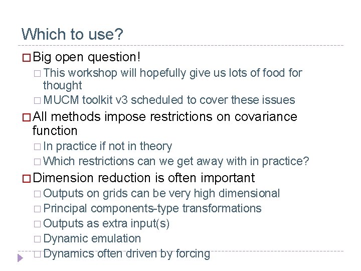
Which to use? � Big open question! � This workshop will hopefully give us lots of food for thought � MUCM toolkit v 3 scheduled to cover these issues � All methods impose restrictions on covariance function � In practice if not in theory � Which restrictions can we get away with in practice? � Dimension � Outputs reduction is often important on grids can be very high dimensional � Principal components-type transformations � Outputs as extra input(s) � Dynamic emulation � Dynamics often driven by forcing

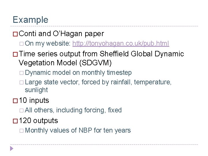
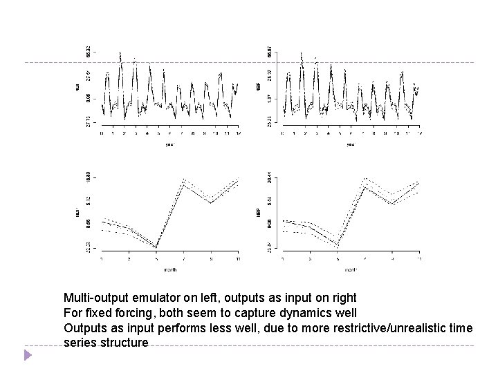
Example � Conti � On and O’Hagan paper my website: http: //tonyohagan. co. uk/pub. html � Time series output from Sheffield Global Dynamic Vegetation Model (SDGVM) � Dynamic model on monthly timestep � Large state vector, forced by rainfall, temperature, sunlight � 10 inputs � All � 120 others, including forcing, fixed outputs � Monthly values of NBP for ten years

Multi-output emulator on left, outputs as input on right For fixed forcing, both seem to capture dynamics well Outputs as input performs less well, due to more restrictive/unrealistic time series structure

Conclusions � Draw your own!