Network simulation Lecture 8 Emulation vs simulation Emulation

Network simulation Lecture 8

Emulation vs. simulation • Emulation: the functioning of a device or of a system is replicated as close to reality as possible – Usually the emulated system can be replaced with the emulating system • The real (i. e. emulated) system is usually faster then the emulating system • Example: emulation of a microprocessor – Network emulation • Is realized in general by describing (in formal language or another formalism) of the protocols involved, according to the specifications that describe these protocols • Simulation: the functioning of a device or system is described at a more abstract and less precise level of representation – Some properties of the system are emphasised and hence included into the simulation model – While other properties, which do not seem to influence (too much) the investigated performance issues, are neglected • Example: if we are interested in the performance of some algorithms used at data link level (e. g. scheduling algorithms), we may neglect some (properties of) higher level protocols (transport, application) or users’ mobility in a mobile network. • However, the aspects that we do not include in the simulation model may have an influence on the performance in a real-life system (e. g. , in mobile data networks, the TCP transport protocolul interract, not always in a fortunate manner, with the lower level protocols

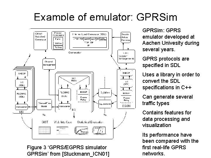
Example of emulator: GPRSim: GPRS emulator developed at Aachen Univesity during several years. GPRS protocols are specified in SDL Uses a library in order to convert the SDL specifications in C++ Can generate several traffic types Contains features for data processing and visualization Figure 3 ‘GPRS/EGPRS simulator GPRSim’ from [Stuckmann_ICN 01] Its performance have been compared with the first real-life GPRS networks.

Network simulators • Used for simulation models in networking, but also in other domains – Can be modelled production lines (for cars or hamburgers) • For a simulation model, the question is how detailed should it be ? – The answer depends according to the purpose and scope of the model: • Academic: usually less detailed (the model is realized by small teams or even by only one person), focused on the studied problem/problems • Industrial: the degree of complexity (and detail) increases as the model is closer to commercial utilization: from simulation to emulation and then prototype.

Commercial vs. non-commercial simulators • Commercial – Developed by companies in order to be sailed (can be very expensive) – Offer: • • • Performance guarantees Possibly cod generation (C, C++, VHDL, etc. ) from the model Example: SES/Workbench (from Hyperformix), OPNET May have cheap or free academic versions (e. g. OPNET) Utilization courses (training): sometimes their documentation is difficult to use without training ! • Non-commercial (Free) – Usually developed by researchers or in universities for research purposes – Then a community of users/developers is formed • Usually a big community means a more successful simulator ! – Can be : • Of similar performance like the commercial ones • Very popular and accepted by academic community (e. g. to publish the simulation results at scientific conferences and journals) • Examples: ns 2, NS 3, cnet, OMNe. T++, • Can have commercial versions ! (e. g. OMNe. T++)

Simulators: utilization • Some simulators offer modules with predefined functions, that can be parametrized. – Examples: • Data source (generator) modules – Parametrized: data generation rate (probability distribution function, mean value, etc) • Server modules: – Parametrized: service rate (probability distribution function, mean value, etc) – They are easy to use, mostly for simple models and by “nonexperts” (i. e. , people that are not able to write computer programs) – Usually they are very “graphical” (icons that can be parametrized) – If we want to change the functioning of a module, it can be very difficult: • It can be necessary to modify some internal functions, not necessarily well documented! • This happens usually with commercial simulators (example: SES/Workbench)

Simulators: utilization • Other simulators are open source: – Usually they are less “graphical”, although they have some graphical interface • The user has to write code, not only to change some parameters or settings by mouse • Usually the code is in a general-purpose programming language (C++, Java) • Sometimes the module interconnection is in “text mode” • They are addressed rather to expert users, capable to write computer programms • If necessary, even the basic functions can be modified (e. g. , the simulation kernel), but this can be a laborious and even risky thing • Usually they have examples of modules (generator, server, sink, etc. ), whose code can be modified or extended. • Example: OMNe. T++ • Simulators close to emulators (ns 2, NS 3 ): – Implement existing protocols (e. g. TCP, IP, UDP, etc) or modules (routers, switches, etc) in some internal format – The simulation model “assembles” these protocols or modules – Can produce long, but very precise simulations, whose results are easily accepted by the scientific community – May have limitations (a certain protocol, module, etc, is not yet implemented). – OMNe. T++ has frameworks that implement protocols (MANET, INET) • Didactic simulators (cnet): simplified, hard to extend, difficult to write programmes (models).

Random numbers • Simulators include random number generators – different probability distribution functions (e. g. uniform, exponential, etc) are provided – Usually the numbers generated are pseudo-random: they are generated by software tools, and they repeat after a very large number of generated values – When simulation repeats, the same “random” numbers are generated! • This is useful in order to compare the results from different simulations • If we want to change the set of generated random numbers, this has to be specified explicitly, by choosing a different seed for the algorithm that generate random numbers

Simulation results • Most simulators have tools for processing simulation results – Statistical values can be collected: mean, minimum and maximum values, standard deviation, number of samples, etc – Can collect traces: all values taken by a parameter (delay, number of lost packets, etc. ) during simulation or during certain time intervals • The traces can be visualized by built-in tools, or by general-purpose tools (gnuplot, Excel, etc) • Resulted trace files can be very big ! – For some simulators, internal format of the files with results (traces, statistics) are simulator-specific (although of text type in general) and need post-processing (with Pearl, etc) – Might be more convenient to collect the results in the format that we want and then to process the results (with gnuplot, Excel, etc).

Validating the simulation results • First we set up the simulation model and check its correctness – Use the graphical interface to visualize different simulation scenarios – Watch the evolution of different parameters (packet delay, number of lost packets, etc) – It is recommended to display many messages like “arrived in module X, the value of the parameter Y is …” – Build deterministic scenarios (avoid random numbers) at the beginning – Imagine different simulation scenarios, including extreme situations (all queues are empty, what does the scheduling algorithm do in this case? ) – Remove errors, until the model works as we wish • Usually these simulations, used to set up the model, are not very long – It means that it is possible that some errors will appear only for longer simulations !

Validating the simulation results • Then collect simulation results – Usually work in “batch” mode, not graphical – Remove unnecessary messages (e. g. , that were used for debugging in previous stages), because they slow down the simulation – Run long simulations, to see if the model is stable – See if the simulation results make sense ! – If they don’t, maybe there are errors in the model – Remove errors, if they appear in this stage (usually they do !!!) – These errors can be hard to debug, e. g. those related to memory allocation • The errors can show up at different simulation moments, depending if we work in graphical mode or not ! – Test the model for extreme situations (e. g. very high network load), but take care to be still stable • Example of unstable system: if a server having an infinite queue receives data at a higher rate than its own service rate, then the queue will grow in time, and hence the packet queueing time will grow as the simulation progresses. In this case the mean value of the delays will be meaningless (bigger for longer simulations)

Confidence in simulation results • • If we have a result like “the average value of packets delay is x”, can we trust this result ? Or, in other words, is the simulation “long enough” ? – Empiric, not very reliable method: run a simulation for a duration T (T is simulation time), and then for 2 T; if the results are “close” then probably the simulation is long enough. – It is desirable to use confidence intervals – Or at least to run a big number of simulations (> 10 or tens of simulations) with different random numbers (take care to avoid overlapping the sets of random numbers) and compare the simulation results, to see if they are “close”. • It is important to use probability distribution functions suitable for the modelled situations, or, if possible, sets of real data – There are trafic types (e. g. video streaming) that cannot be modelled by probability distribution functions • • If there appear anomalies (e. g. the graphic of a parameter has an increasing trend, but there is a region where the values decrease), try to find an explanation. The anomalies can be caused by errors in the model, but not necessarily: – E. g. , if there are certain relations between numbers, like for round robin type scheduling algorithms, or, more generally, relations between integer numbers.

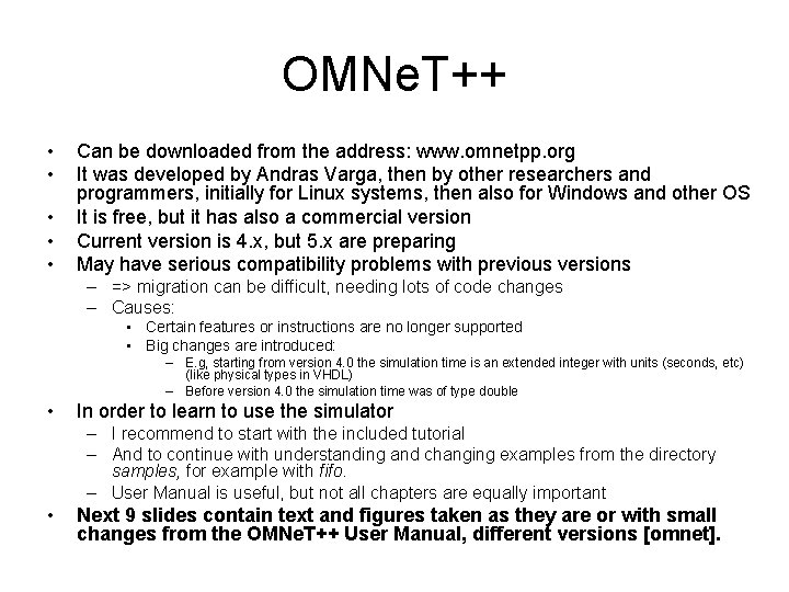
OMNe. T++ • • • Can be downloaded from the address: www. omnetpp. org It was developed by Andras Varga, then by other researchers and programmers, initially for Linux systems, then also for Windows and other OS It is free, but it has also a commercial version Current version is 4. x, but 5. x are preparing May have serious compatibility problems with previous versions – => migration can be difficult, needing lots of code changes – Causes: • Certain features or instructions are no longer supported • Big changes are introduced: – E. g, starting from version 4. 0 the simulation time is an extended integer with units (seconds, etc) (like physical types in VHDL) – Before version 4. 0 the simulation time was of type double • In order to learn to use the simulator – I recommend to start with the included tutorial – And to continue with understanding and changing examples from the directory samples, for example with fifo. – User Manual is useful, but not all chapters are equally important • Next 9 slides contain text and figures taken as they are or with small changes from the OMNe. T++ User Manual, different versions [omnet].

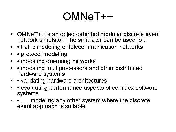
OMNe. T++ • OMNe. T++ is an object-oriented modular discrete event network simulator. The simulator can be used for: • • traffic modeling of telecommunication networks • • protocol modeling • • modeling queueing networks • • modeling multiprocessors and other distributed hardware systems • • validating hardware architectures • • evaluating performance aspects of complex software systems • • . . . modeling any other system where the discrete event approach is suitable.

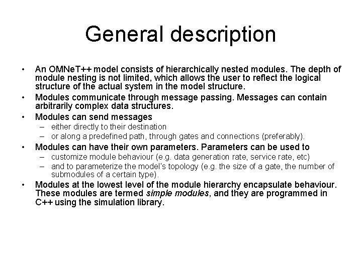
General description • • • An OMNe. T++ model consists of hierarchically nested modules. The depth of module nesting is not limited, which allows the user to reflect the logical structure of the actual system in the model structure. Modules communicate through message passing. Messages can contain arbitrarily complex data structures. Modules can send messages – either directly to their destination – or along a predefined path, through gates and connections (preferably). • Modules can have their own parameters. Parameters can be used to – customize module behaviour (e. g. data generation rate, service rate, etc) – and to parameterize the model’s topology (e. g. the size of a gate, the number of submodules of a certain type). • Modules at the lowest level of the module hierarchy encapsulate behaviour. These modules are termed simple modules, and they are programmed in C++ using the simulation library.

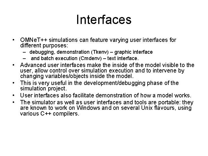
Interfaces • OMNe. T++ simulations can feature varying user interfaces for different purposes: – debugging, demonstration (Tkenv) – graphic interface – and batch execution (Cmdenv) – text interface. • Advanced user interfaces make the inside of the model visible to the user, allow control over simulation execution and to intervene by changing variables/objects inside the model. • This is very useful in the development/debugging phase of the simulation project. • User interfaces also facilitate demonstration of how a model works. • The simulator as well as user interfaces and tools are portable: they are known to work on Windows and on several Unix flavours, using various C++ compilers.

Modeling concepts • OMNe. T++ provides efficient tools for the user to describe the structure of the actual system. Some of the main features are: • • hierarchically nested modules • • modules are instances of module types • • modules communicate with messages through channels • • flexible module parameters • • topology description language

Hierarchical modules • An OMNe. T++ model consists of hierarchically nested modules, which communicate by passing messages to each another. • OMNe. T++ models are often referred to as networks. • The top level module is the system module. The system module contains submodules, which can also contain submodules themselves • The depth of module nesting is not limited; this allows the user to reflect the logical structure of the actual system in the model structure. – See figure: • Model structure is described in OMNe. T++’s NED language.

Simple and compound modules Figure taken from [omnet]

Simple modules in OMNe. T++ • In OMNe. T++, events occur inside simple modules. Simple modules encapsulate C++ code that generates events and reacts to events, in other words, implements the behaviour of the model. • The user creates simple module types by subclassing the c. Simple. Module class, which is part of the OMNe. T++ class library. • c. Simple. Module, just as c. Compound. Module, is derived from a common base class, c. Module. • c. Simple. Module, although packed with simulation-related functionality, doesn’t do anything useful by itself – you have to redefine some virtual member functions to make it do useful work. • These member functions are the following: • • void initialize() • • void handle. Message(c. Message *msg) • • void activity() • • void finish()

Functions • In the initialization step, OMNe. T++ builds the network: it creates the necessary simple and compound modules and connects them according to the NED definitions. OMNe. T++ also calls the initialize() functions of all modules. • The handle. Message() and activity() functions are called during event processing. • This means that the user will implement the model’s behavior in these functions. • handle. Message() and activity() implement different event processing strategies: for each simple module, the user has to redefine exactly one of these functions. (not both !)

Functions (cont’d) • handle. Message() is a method that is called by the simulation kernel when the module receives a message. • activity() is a coroutine-based solution which implements the process interaction approach • coroutines are non-preemptive (i. e. cooperative) threads. • Generally, it is recommended that you prefer handle. Message() to activity() – mainly because activity() doesn’t scale well (you have to reserve stack for each module that uses activity()). • Modules written with activity() and handle. Message() can be freely mixed within a simulation model. • The finish() functions are called when the simulation terminates successfully. • The most typical use of finish() is the recording of statistics collected during simulation.

Communication between modules • Many times it is necessary to read (and maybe to modify) in a module information form other modules – E. g. a module named scheduler wants to know the length of the queues from the “user” modules • Can be done in 3 ways: 1. Using global variables 2. Using OMNe. T++ messages 3. Using modules parameters

Communication between modules 1. Using global variables – Advantages: efficient regarding the duration of simulation – Drawbacks: • Easy to make synchronization errors when accessing the global variables • Results an ugly code • 2. Using OMNe. T++ messages – Advantages: is closer to reality – Drawbacks: • Increases simulator load and increases the duration of simulation • There appear too many “types” of messages: – Messages that represent data in a real system (packets, blocks of data, etc) – Messages that represent important signaling in a real system (e. g. command given by the scheduler to transmit a certain number of data blocks from a user’s buffer) – Messages that represent information transmitted ( e. g. the length of a queue, etc. )

Communication between modules • 3. Using parameters – Advantages: • Clear distinction between data exchange and signaling between modules • Safer than with global variables – Drawbacks: • long(er) code: first change a value from a module (e. g. the variable that stores the queue length), then change the module parameter that store this value, then another module reads this value

Example of simulation models • 1. Simulation model for vertical handover (VHO) • 2. Simulation model for resource allocation in a GPRS/EGPRS network

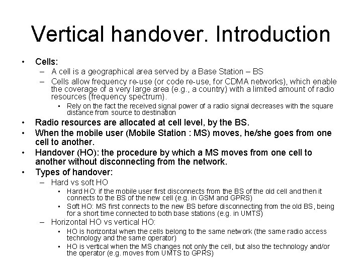
Vertical handover. Introduction • Cells: – A cell is a geographical area served by a Base Station – BS – Cells allow frequency re-use (or code re-use, for CDMA networks), which enable the coverage of a very large area (e. g. , a country) with a limited amount of radio resources (frequency spectrum). • Rely on the fact the received signal power of a radio signal decreases with the square distance from source to destination • • Radio resources are allocated at cell level, by the BS. When the mobile user (Mobile Station : MS) moves, he/she goes from one cell to another. Handover (HO): the procedure by which a MS moves from one cell to another without disconnecting from the network. Types of handover: – Hard vs soft HO • Hard HO: if the mobile user first disconnects from the BS of the old cell and then it connects to the BS of the new cell (e. g. in GSM and GPRS) • Soft HO: MS first connects to the new BS before disconnecting from the old BS, being for a short time connected to both base stations (e. g. in UMTS) – Horizontal HO vs vertical HO: • HO is horizontal when the cells belong to the same network (the same radio access technology and the same operator) • HO is vertical when the MS changes not only the cell, but also the technology and/or the operator (e. g. moves from UMTS to GPRS)

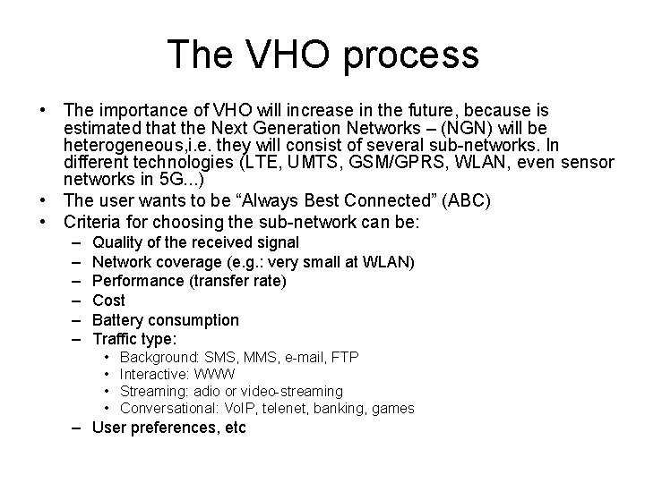
The VHO process • The importance of VHO will increase in the future, because is estimated that the Next Generation Networks – (NGN) will be heterogeneous, i. e. they will consist of several sub-networks. In different technologies (LTE, UMTS, GSM/GPRS, WLAN, even sensor networks in 5 G. . . ) • The user wants to be “Always Best Connected” (ABC) • Criteria for choosing the sub-network can be: – – – Quality of the received signal Network coverage (e. g. : very small at WLAN) Performance (transfer rate) Cost Battery consumption Traffic type: • • Background: SMS, MMS, e-mail, FTP Interactive: WWW Streaming: adio or video-streaming Conversational: Vo. IP, telenet, banking, games – User preferences, etc

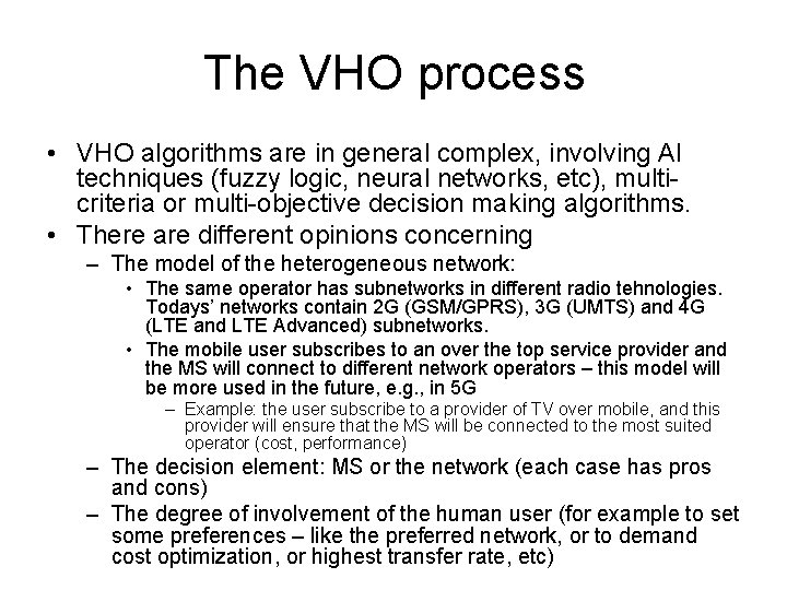
The VHO process • VHO algorithms are in general complex, involving AI techniques (fuzzy logic, neural networks, etc), multicriteria or multi-objective decision making algorithms. • There are different opinions concerning – The model of the heterogeneous network: • The same operator has subnetworks in different radio tehnologies. Todays’ networks contain 2 G (GSM/GPRS), 3 G (UMTS) and 4 G (LTE and LTE Advanced) subnetworks. • The mobile user subscribes to an over the top service provider and the MS will connect to different network operators – this model will be more used in the future, e. g. , in 5 G – Example: the user subscribe to a provider of TV over mobile, and this provider will ensure that the MS will be connected to the most suited operator (cost, performance) – The decision element: MS or the network (each case has pros and cons) – The degree of involvement of the human user (for example to set some preferences – like the preferred network, or to demand cost optimization, or highest transfer rate, etc)

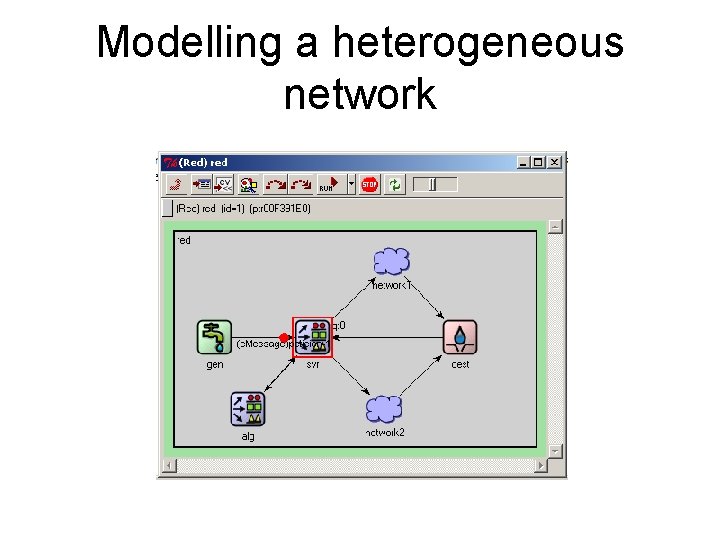
Modelling the VHO process • The main problem for modelling is the different time granularity of the events: – Scheduling in a mobila network is made at time intervals of milli seconds (1 ms in LTE, 10 ms in UMTS, 20 ms in GPRS) – Data packets (e. g. IP packets) are generated at intervals of seconds – Selecting of a different cell (possibly from another sub-network) takes place at intervals of tens of seconds or even minutes • If we model at the scheduling level (ms), then the resulted simulations will be very long • Another possibility is to model at the IP packet level: – Consider the IP packet length of 1000 – 1500 Bytes and we estimate/compute the duration of the transmission of an IP packet IP in different networks, according to different load and radio conditions. • It results the following simulation model:

Modelling a heterogeneous network

Modelling a heterogeneous network • Explanations: – gen: data generator, which generates OMNe. T messages at certain time intervals. The mesages represent files, of certain length, application dependent – svr: server • Stores in queues the files created by the generator • The queues can be per user, per user classes, traffic types , both for downlink - DL and for UL – uplink • Transmits a file in the network chosen by the module alg. – alg: the algorithm that selects the sub-network – dest: destination • node of type sink, colects statistics and deletes the mesages • Informes the server when a file has been transmitted completly so that the server can transmit the next file – Network 1, Network 2: two sub-networks, for example one UMTS and one GPRS. The model of such a sub-network is detailed on the next slide:

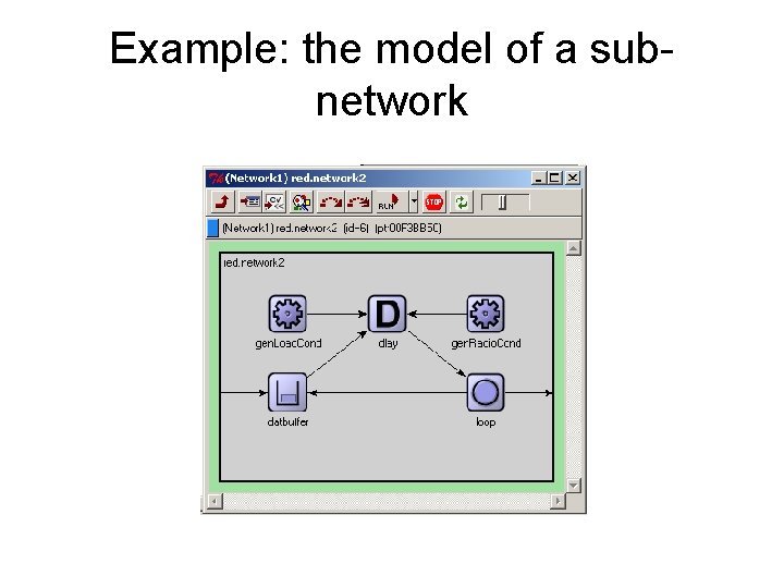
Example: the model of a subnetwork

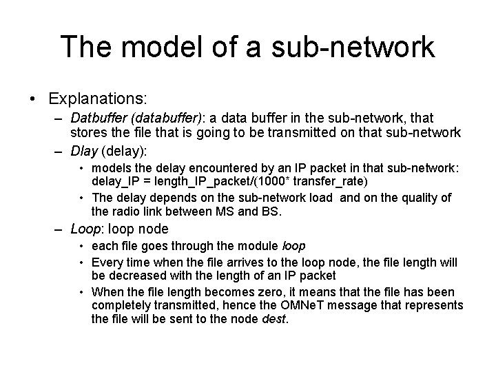
The model of a sub-network • Explanations: – Datbuffer (databuffer): a data buffer in the sub-network, that stores the file that is going to be transmitted on that sub-network – Dlay (delay): • models the delay encountered by an IP packet in that sub-network: delay_IP = length_IP_packet/(1000* transfer_rate) • The delay depends on the sub-network load and on the quality of the radio link between MS and BS. – Loop: loop node • each file goes through the module loop • Every time when the file arrives to the loop node, the file length will be decreased with the length of an IP packet • When the file length becomes zero, it means that the file has been completely transmitted, hence the OMNe. T message that represents the file will be sent to the node dest.

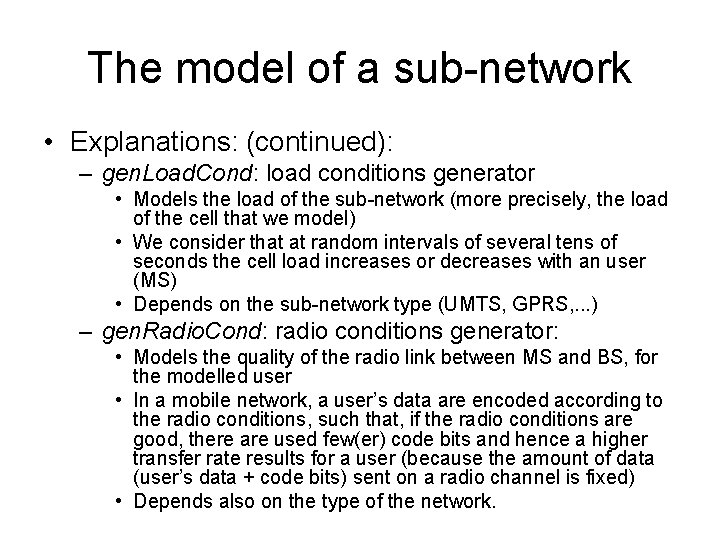
The model of a sub-network • Explanations: (continued): – gen. Load. Cond: load conditions generator • Models the load of the sub-network (more precisely, the load of the cell that we model) • We consider that at random intervals of several tens of seconds the cell load increases or decreases with an user (MS) • Depends on the sub-network type (UMTS, GPRS, . . . ) – gen. Radio. Cond: radio conditions generator: • Models the quality of the radio link between MS and BS, for the modelled user • In a mobile network, a user’s data are encoded according to the radio conditions, such that, if the radio conditions are good, there are used few(er) code bits and hence a higher transfer rate results for a user (because the amount of data (user’s data + code bits) sent on a radio channel is fixed) • Depends also on the type of the network.

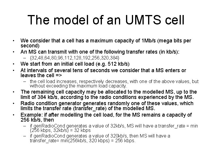
The model of an UMTS cell • • We consider that a cell has a maximum capacity of 1 Mb/s (mega bits per second) An MS can transmit with one of the following transfer rates (in kb/s): – {32, 48, 64, 80, 96, 112, 128, 192, 256, 320, 384} • • We start from an initial cell load (e. g. 512 kb/s) At intervals of several tens of seconds we consider that a MS enters or leaves the cell => – the cell load increases, respectively decreases, with one of the above values, but without exceeding the maximum load capacity. • • • The remaining cell capacity may be allocated to the modelled MS, up to the limit of 384 kb/s, according to the radio conditions experienced by the MS. Radio condition generator generates randomly one of these values, which limits the transfer rate (transfer_rate) of the modelled MS. Example: if after modelling the cell load, for the MS remains a capacity of 256 kb/s, then – if gen. Radio. Cond generates a value of 32 kb/s, MS will have a transfer_rate = min (256 kbps, 32 kb/s) = 32 kbps – if gen. Radio. Cond generates a value of 320 kb/s, then MS will have a transfer_rate= min(256 kb/s, 320 kbps) = 256 kbps.

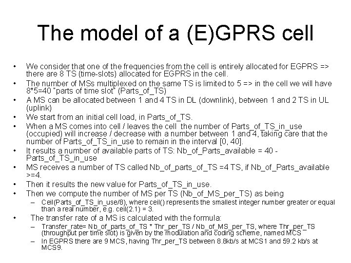
The model of a (E)GPRS cell • • • We consider that one of the frequencies from the cell is entirely allocated for EGPRS => there are 8 TS (time-slots) allocated for EGPRS in the cell. The number of MSs multiplexed on the same TS is limited to 5 => in the cell we will have 8*5=40 “parts of time slot” (Parts_of_TS) A MS can be allocated between 1 and 4 TS in DL (downlink), between 1 and 2 TS in UL (uplink) We start from an initial cell load, in Parts_of_TS. When a MS comes into cell / leaves the cell the number of Parts_of_TS_in_use (occupied) will increase / decrease with a number between 1 and 4, taking care that the number of Parts_of_TS_in_use to remain in the interval [0, 40]. It results a number of available parts of TS: Nb_of_Parts_available = 40 - Parts_of_TS_in_use MS receives a number of TS called Nb_of_parts_of_TS =4 TS, if Nb_of_Parts_available >=4. Then it results the new value for Parts_of_TS_in_use. Then we compute the number of MS per TS (Nb_of_MS_per_TS) as being – Ceil(Parts_of_TS_in_use/8), where ceil() represents the smallest integer number greater or equal than a real number, e. g. ceil(2. 1) = 3. • The transfer rate of a MS is calculated with the formula: – Transfer_rate= Nb_of_parts_of_TS * Thr_per_TS / Nb_of_MS_per_TS, where Thr_per_TS (throughput per time slot) is given by the modulation and coding scheme, named MCS – In EGPRS there are 9 MCS, having Thr_per_TS between 8. 8 kb/s at MCS 1 and 59. 2 kb/s at MCS 9.

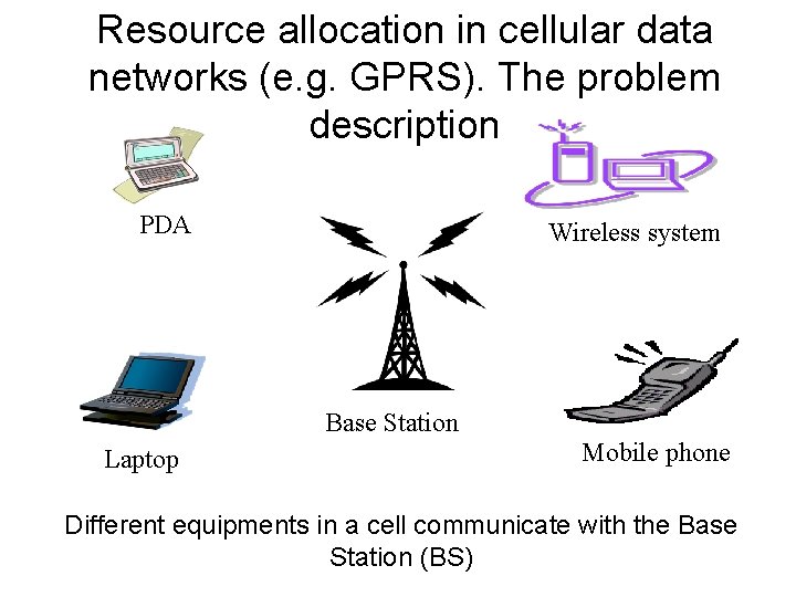
Resource allocation in cellular data networks (e. g. GPRS). The problem description PDA Wireless system Base Station Laptop Mobile phone Different equipments in a cell communicate with the Base Station (BS)

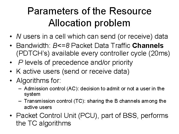
Parameters of the Resource Allocation problem • N users in a cell which can send (or receive) data • Bandwidth: B<=8 Packet Data Traffic Channels (PDTCH’s) available every controller cycle (20 ms) • P levels of precedence and/or priority • K active users (send or receive data) • Algorithms for: – Admission control (AC): decision to admit or not a user in the system – Transmission control (TC): sharing the B channels among the active users • Packet Control Unit (PCU), part of BSS, performs the TC algorithms

user[0] K active users N users in a cell user[1] user[2] user[K-1] user[K] N-K inactive users user[N-1] B=8 PDTCHs every 20 ms

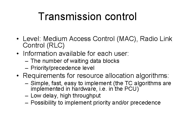
Transmission control • Level: Medium Access Control (MAC), Radio Link Control (RLC) • Information available for each user: – The number of waiting data blocks – Priority/precedence level • Requirements for resource allocation algorithms: – Simple, fast, easy to implement (the TC algorithms are implemented in hardware, i. e. in the PCU) – Low delay, high throughput – Possibility to implement priority and/or precedence

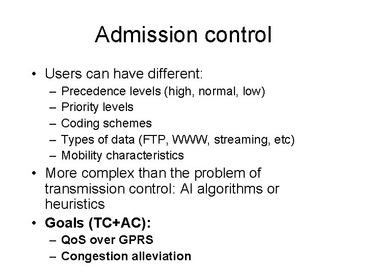
Admission control • Users can have different: – – – Precedence levels (high, normal, low) Priority levels Coding schemes Types of data (FTP, WWW, streaming, etc) Mobility characteristics • More complex than the problem of transmission control: AI algorithms or heuristics • Goals (TC+AC): – Qo. S over GPRS – Congestion alleviation

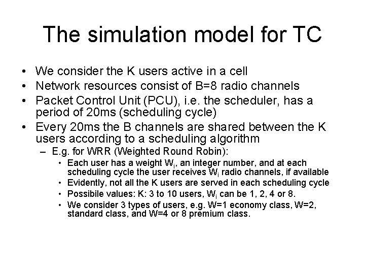
The simulation model for TC • We consider the K users active in a cell • Network resources consist of B=8 radio channels • Packet Control Unit (PCU), i. e. the scheduler, has a period of 20 ms (scheduling cycle) • Every 20 ms the B channels are shared between the K users according to a scheduling algorithm – E. g. for WRR (Weighted Round Robin): • Each user has a weight Wi, an integer number, and at each scheduling cycle the user receives Wi radio channels, if available • Evidently, not all the K users are served in each scheduling cycle • Possibile values: K: 3 to 10 users, Wi can be 1, 2, 4 or 8. • We consider 3 types of users, e. g. W=1 economy class, W=2, standard class, and W=4 or 8 premium class.

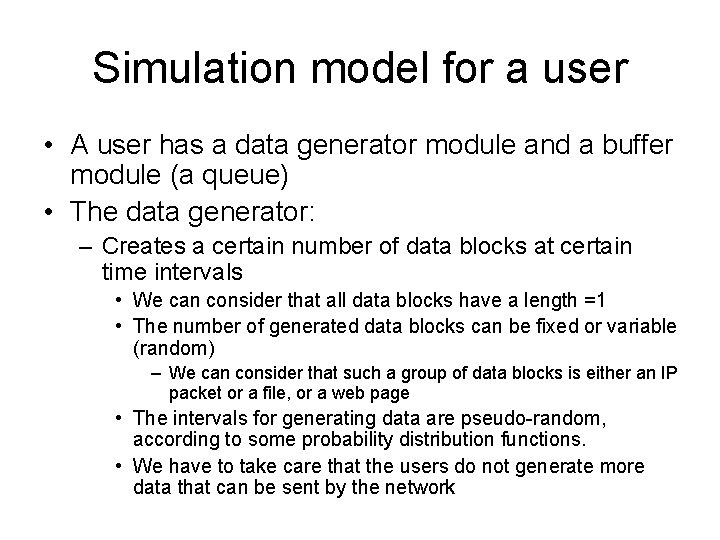
Simulation model for a user • A user has a data generator module and a buffer module (a queue) • The data generator: – Creates a certain number of data blocks at certain time intervals • We can consider that all data blocks have a length =1 • The number of generated data blocks can be fixed or variable (random) – We can consider that such a group of data blocks is either an IP packet or a file, or a web page • The intervals for generating data are pseudo-random, according to some probability distribution functions. • We have to take care that the users do not generate more data that can be sent by the network

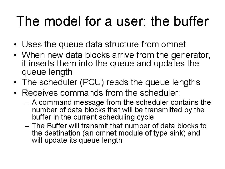
The model for a user: the buffer • Uses the queue data structure from omnet • When new data blocks arrive from the generator, it inserts them into the queue and updates the queue length • The scheduler (PCU) reads the queue lengths • Receives commands from the scheduler: – A command message from the scheduler contains the number of data blocks that will be transmitted by the buffer in the current scheduling cycle – The Buffer will transmit that number of data blocks to the destination (an omnet module of type sink) and will update its queue length

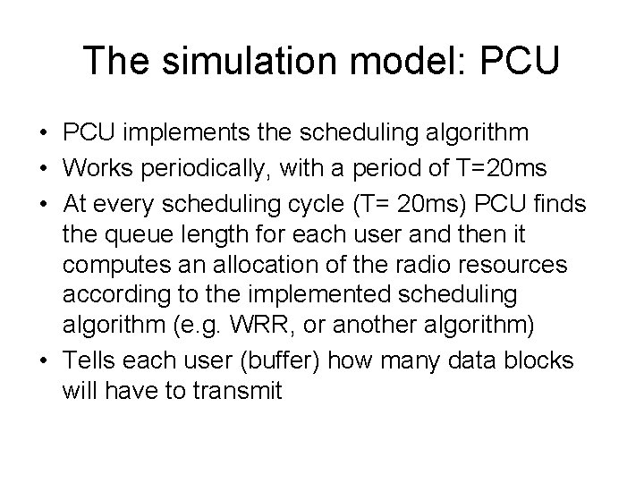
The simulation model: PCU • PCU implements the scheduling algorithm • Works periodically, with a period of T=20 ms • At every scheduling cycle (T= 20 ms) PCU finds the queue length for each user and then it computes an allocation of the radio resources according to the implemented scheduling algorithm (e. g. WRR, or another algorithm) • Tells each user (buffer) how many data blocks will have to transmit

The simulation model: the sink • The module sink represents the destination for data: it collects statistics and deletes the omnet messages. • In theory, each user should have its own sink module • But it is more efficient if there is only one sink for the entire simulation model, because – The sink collects statistics (mean, maximum, minimum values, standard deviations, etc) about the simulation results, and these statistics are easier processed if they are in the same module • Will have one input for each user • Will have to compute the transmission delays for each data packet (or file, or web page) • Statistics can be per user, per user class, etc. • Can collect also trace-es for (certain) users: e. g. the evolution in time of the packets delays for a user (during a simulation time interval)

The simulation model • May contain other modules: – E. g. a module to model the radio conditions: when they are very bad, certain data blocks are lost and have to be re-transmitted – A module that models the voice traffic in the GPRS cell: it modifies randomly the number of channels B in order to model the channels allocated to voice traffic • This simulation model is obviously very simplified compared to a real (E)GPRS network, but it is still realistic. • The AC is not included in the model, in order to avoid increasing too much its complexity.

Bibliography • [omnet] OMNe. T++ User Manual, Version 4. 1. Andras Varga and Open. Sim Ltd, 2010. [Online]. Available: http: //www. omnetpp. org/ • [Stuckmann_ICN 01] Stuckmann, Peter, and Frank Müller. "Quality of service management in GPRS networks. " Networking—ICN 2001. Springer Berlin Heidelberg, 2001. 276 -285.