Further Stats 1 Chapter 6 ChiSquared Tests jfrosttiffin

Further Stats 1 Chapter 6 : : Chi-Squared Tests jfrost@tiffin. kingston. sch. uk www. drfrostmaths. com @Dr. Frost. Maths Last modified: 23 rd July 2018

www. drfrostmaths. com Everything is completely free. Why not register? Register now to interactively practise questions on this topic, including past paper questions and extension questions (including MAT + UKMT). Teachers: you can create student accounts (or students can register themselves), to set work, monitor progress and even create worksheets. With questions by: Dashboard with points, trophies, notifications and student progress. Questions organised by topic, difficulty and past paper. Teaching videos with topic tests to check understanding.

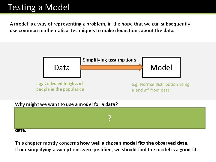
Testing a Model A model is a way of representing a problem, in the hope that we can subsequently use common mathematical techniques to make deductions about the data. Data Simplifying assumptions Model e. g. Collected heights of people in the population Why might we want to use a model for a data? It often makes calculations from the data easier, e. g. for heights in the population, if we assume a Normal Distribution, we could ? then calculate probabilities of someone having a given height range. This might be difficult if we used the raw data. This chapter mostly concerns how well a chosen model fits the observed data. If our simplifying assumptions were justified, we should find the model is a good fit.

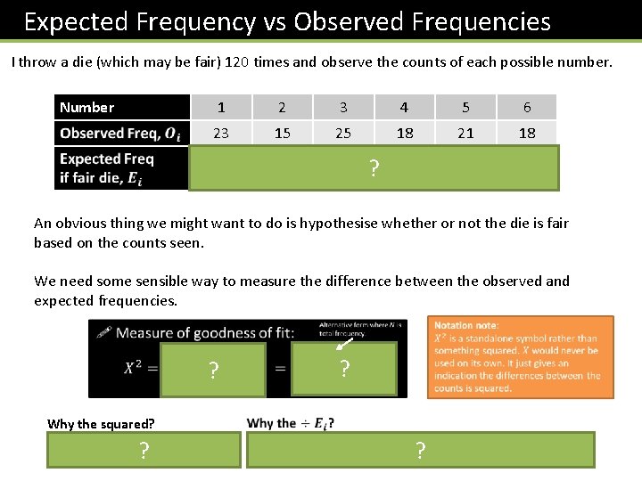
Expected Frequency vs Observed Frequencies I throw a die (which may be fair) 120 times and observe the counts of each possible number. Number 1 2 3 4 5 6 23 15 25 18 21 18 20 20 20 ? An obvious thing we might want to do is hypothesise whether or not the die is fair based on the counts seen. We need some sensible way to measure the difference between the observed and expected frequencies. ? Why the squared? It ensures difference is positive. ? ? ?

Example [Textbook] Billy and Mel each have two 4 -sided spinners numbered 1 -4. They each carry out experiments, where they spin their spinners at the same time, and add the scores together. After each student has carried out 160 experiments, the frequency distributions are as follows: 12 15 22 41 33 21 16 6 12 21 37 35 29 20 10 20 30 40 30 20 10 Both Billy and Mel believe that their spinners are fair. (a) State the null and alternative hypotheses for the experiment. One of the students has a biased spinner. (b) Calculate the goodness of fit for both students, and determine which of them is most likely to have the biased spinner. ? a ? b

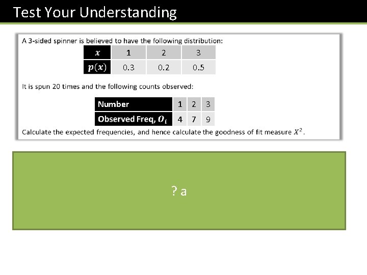
Test Your Understanding 1 2 3 0. 2 0. 5 Number 1 2 3 4 7 9 6 4 10 1 2 3 4 7 9 ? a

Exercise 6 A Pearson Further Statistics 1 Pages 95 -96

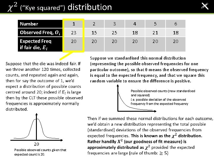
! Number 1 2 3 4 5 6 23 15 25 18 21 18 20 20 20 Suppose we standardised this normal distribution (representing the possible observed frequencies for one particular outcome), so that 0 means the observed frequency is equal to the expected frequency, and that we square this random variable to ensure the difference is positive. Possible observed counts (now standardised and squared) i. e. possible deviation of the observed frequency from the expected frequency Possible observed counts given that expected count is 20.

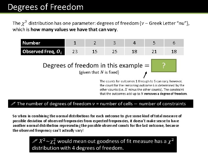
Degrees of Freedom Number 1 2 3 4 5 6 23 15 25 18 21 18 ? So when in combining the normal distributions for each outcome to give some kind of total measure of possible deviation of observed frequencies from expected frequencies, it doesn’t make sense to have another normal distribution representing the possible observed counts for the last outcome, because the observed frequency can’t actually vary!

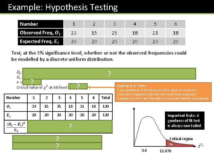
Example: Hypothesis Testing Number 1 2 3 4 5 6 23 15 25 18 21 18 20 20 20 Test, at the 5% significance level, whether or not the observed frequencies could be modelled by a discrete uniform distribution. ? ? Number ? 1 2 3 4 5 6 Total 23 15 25 18 21 18 120 20 120 0. 45 1. 25 0. 2 0. 05 0. 2 3. 4 ? ? ? Important Note: A goodness of fit test is always one-tailed. Critical region 5% 3. 4 11. 070

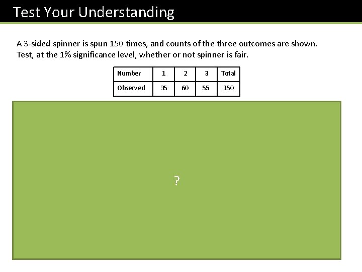
Test Your Understanding A 3 -sided spinner is spun 150 times, and counts of the three outcomes are shown. Test, at the 1% significance level, whether or not spinner is fair. Number 1 2 3 Total Observed 35 60 55 150 ? 1 2 3 Total 35 60 55 150 50 150 4. 5 2 0. 5 7

Exercise 6 C Pearson Further Statistics 1 Pages 102 -103 (These slides skipped Exercise 6 B)

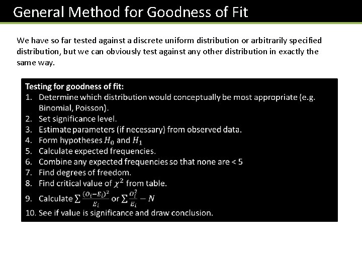
General Method for Goodness of Fit We have so far tested against a discrete uniform distribution or arbitrarily specified distribution, but we can obviously test against any other distribution in exactly the same way.

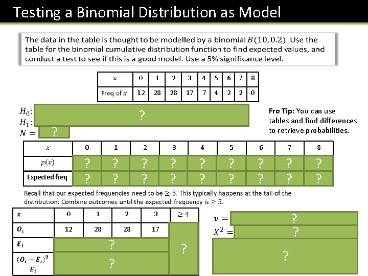
Testing a Binomial Distribution as Model 0 1 2 3 4 5 6 7 8 12 28 28 17 7 4 2 2 0 Fro Tip: You can use tables and find differences to retrieve probabilities. ? ? 0 1 2 3 4 5 6 7 8 ? 10. 75 ? 0. 2684 ? 26. 84 ? 0. 3020 ? 30. 20 ? 0. 2013 ? 20. 13 ? 0. 0881 ? 8. 81 ? 0. 0264 ? 2. 64 ? 0. 0055 ? 0. 55 ? 0. 0008 ? 0. 08 ? 0. 0001 0. 1074 Expected freq 0 1 2 3 12 28 28 17 15 20. 13 12. 09 0. 4867 0. 7004 10. 74 0. 1478 ? 30. 20 0. 0501 0. 1603 ? 26. 84 ? ? ? ? ? 0. 01 ?

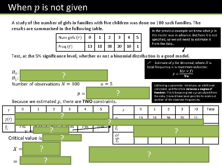
A study of the number of girls in families with five children was done on 100 such families. The results are summarised in the following table. 0 1 2 3 4 5 13 18 38 20 10 1 Test, at the 5% significance level, whether or not a binomial distribution is a good model. ? ? 0 1 2 0. 0791 0. 2614 0. 3456 ? 0. 2285 7. 91 26. 14 34. 56 22. 85 ? ? ? 3 ? 4 5 0 1 2 3 >3 0. 0755 0. 0099 13 18 38 20 11 7. 55 0. 99 7. 91 26. 14 34. 56 22. 85 8. 54 21. 37 12. 39 41. 78 ? ? ? 17. 51 14. 17 Total 107. 22

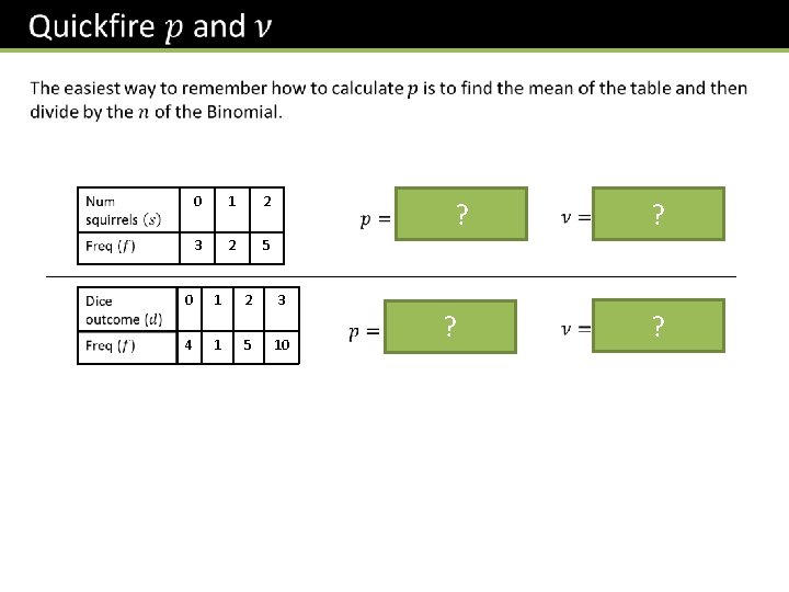
0 1 2 3 2 5 ? 0 1 2 3 4 1 5 10 ? ? ?

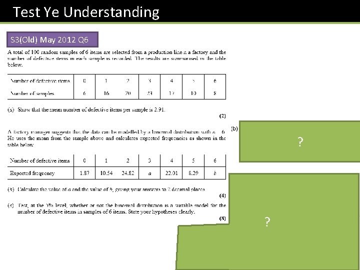
Test Ye Understanding S 3(Old) May 2012 Q 6 ? ?

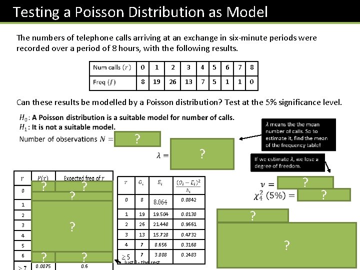
Testing a Poisson Distribution as Model The numbers of telephone calls arriving at an exchange in six-minute periods were recorded over a period of 8 hours, with the following results. 0 1 2 3 4 5 6 7 8 8 19 26 13 7 5 1 1 0 Can these results be modelled by a Poisson distribution? Test at the 5% significance level. ? 0. 1108 ? 0 8 21. 448 1 19 19. 504 0. 0130 15. 728 2 26 21. 448 0. 9661 8. 656 3 13 15. 728 0. 4732 4 7 8. 656 0. 3168 7 3. 808 0. 2483 0. 2438 2 0. 2681 3 0. 1966 4 0. 1082 5 0. 0476 3. 808 6 0. 0174 1. 392 0. 0075 0. 6 ? ? ? 19. 504 ? 0. 0842 Just 1 - the rest. ? ? ?

Exercise 6 D Pearson Further Statistics 1 Pages 110 -113

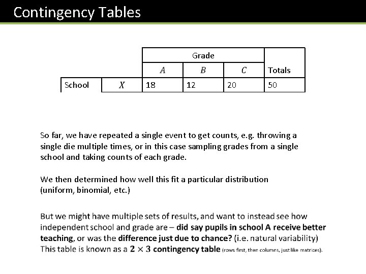
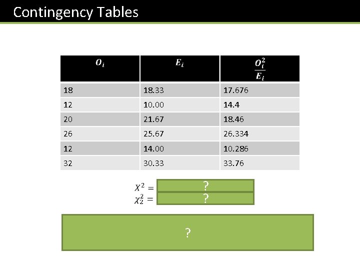
Contingency Tables Grade Totals School Totals 18 12 20 50 26 12 32 70 44 24 52 120 So far, we have repeated a single event to get counts, e. g. throwing a single die multiple times, or in this case sampling grades from a single school and taking counts of each grade. We then determined how well this fit a particular distribution (uniform, binomial, etc. )

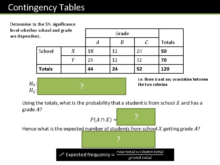
Contingency Tables Determine to the 5% significance level whether school and grade are dependent. Grade Totals School Totals 18 12 20 50 26 12 32 70 44 24 52 120 i. e. there is not any association between the two criterion ? ? ?

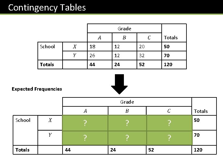
Contingency Tables Grade Totals School Totals 18 12 20 50 26 12 32 70 44 24 52 120 Expected Frequencies Grade Totals School Totals 44 ? ? ? 50 ? ? ? 70 24 52 120

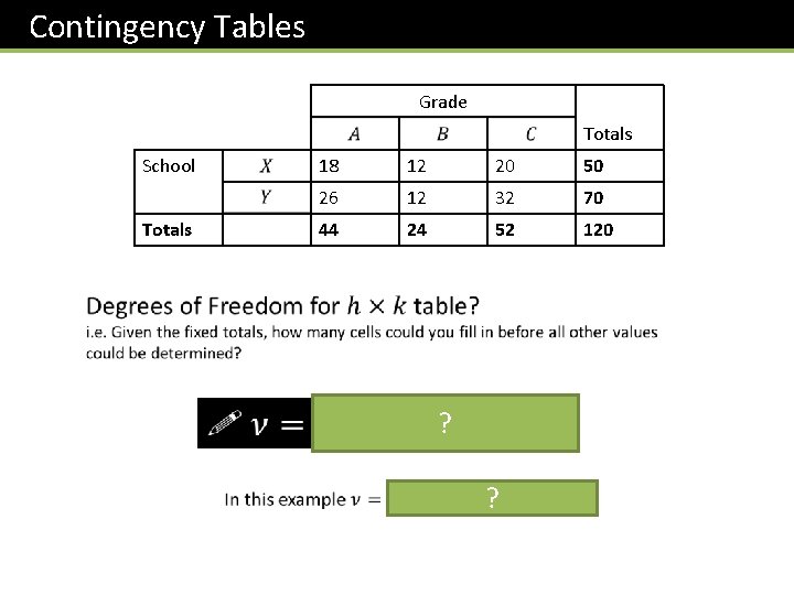
Contingency Tables Grade Totals School Totals 18 12 20 50 26 12 32 70 44 24 52 120 ? ?

Contingency Tables 18 18. 33 17. 676 12 10. 00 14. 4 20 21. 67 18. 46 26 25. 67 26. 334 12 14. 00 10. 286 32 30. 33 33. 76 ? ? ?

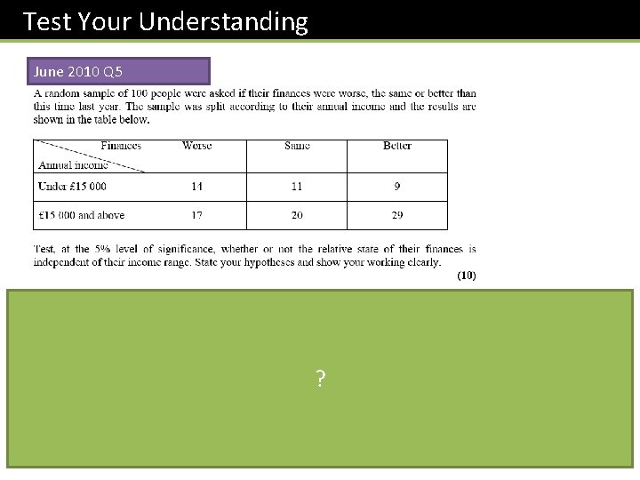
Test Your Understanding June 2010 Q 5 ?

Exercise 6 E Pearson Further Statistics 1 Pages 116 -119

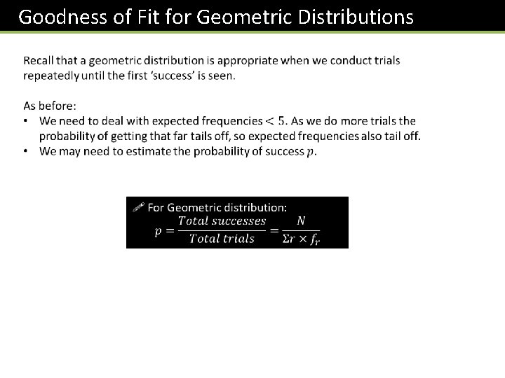
Goodness of Fit for Geometric Distributions

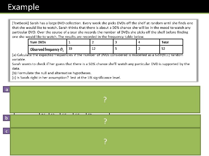
Example Num DVDs a b 1 2 3 4 Total 33 12 5 2 52 1 2 3 Total 33 12 5 2 0. 5 0. 25 0. 125 26 13 6. 5 52 52 ? ? c ? The highest observed outcome was 4. Since the geometric distribution has infinite outcomes, we treat 4 as “ 4 or more”. The last expected frequency will therefore be 52 minus the others.

Exercise 6 F Pearson Further Statistics 1 Pages 121 -122