ForwardLooking Market Risk Premium Weiqi Zhang National University

Forward-Looking Market Risk Premium Weiqi Zhang National University of Singapore Dec 2010

Background Estimating risk premium • Historical average of realized excess returns – Backward-looking – The risk premium estimate can be negative even using an estimation period of 10 years (from 1973 to 1984) • Forward-looking risk premium – Our new approach is based on option prices (Relate forward-looking market risk premium to (1) investors’ risk aversion implied by the option market, and (2) forward-looking physical moments – variance, skewness and kurtosis)

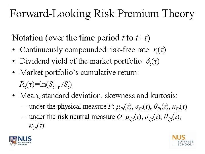
Forward-Looking Risk Premium Theory Notation (over the time period t to t+τ) • Continuously compounded risk-free rate: rt(τ) • Dividend yield of the market portfolio: δt(τ) • Market portfolio’s cumulative return: Rt(τ)=ln(St+τ /St) • Mean, standard deviation, skewness and kurtosis: – under the physical measure P: μPt(τ), σPt(τ), θPt(τ), κPt(τ) – under the risk neutral measure Q: μQt(τ), σQt(τ), θQt(τ), κQt(τ)

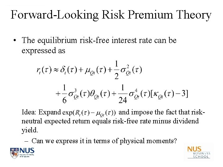
Forward-Looking Risk Premium Theory • The equilibrium risk-free interest rate can be expressed as Idea: Expand impose the fact that riskneutral expected return equals risk-free rate minus dividend yield. – Can we express it in terms of physical moments?

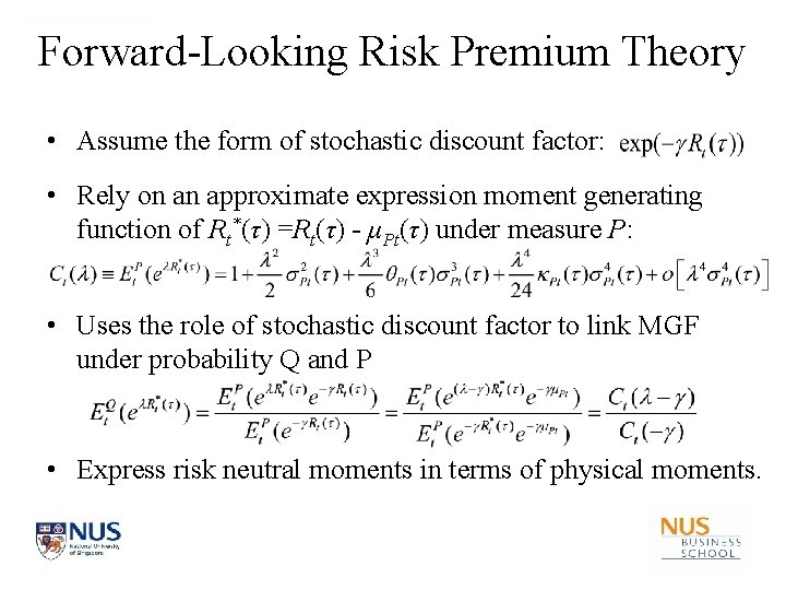
Forward-Looking Risk Premium Theory • Assume the form of stochastic discount factor: • Rely on an approximate expression moment generating function of Rt*(τ) =Rt(τ) - μPt(τ) under measure P: • Uses the role of stochastic discount factor to link MGF under probability Q and P • Express risk neutral moments in terms of physical moments.

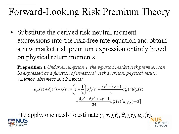
Forward-Looking Risk Premium Theory • Substitute the derived risk-neutral moment expressions into the risk-free rate equation and obtain a new market risk premium expression entirely based on physical return moments: Proposition 1 Under Assumption 1, the τ-period market risk premium can be expressed as a function of investors’ risk aversion, physical return variance, skewness and kurtosis: To apply, one needs to estimate γ, σPt(τ), θPt(τ), κPt(τ).

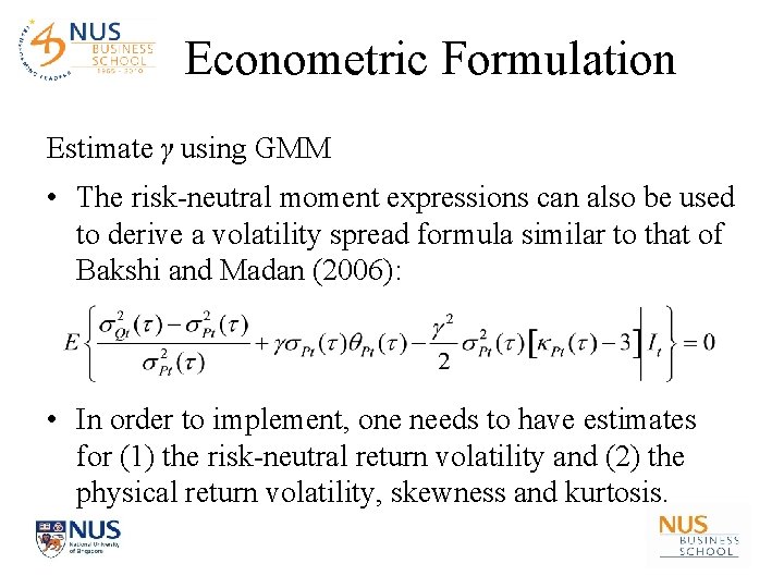
Econometric Formulation Estimate γ using GMM • The risk-neutral moment expressions can also be used to derive a volatility spread formula similar to that of Bakshi and Madan (2006): • In order to implement, one needs to have estimates for (1) the risk-neutral return volatility and (2) the physical return volatility, skewness and kurtosis.

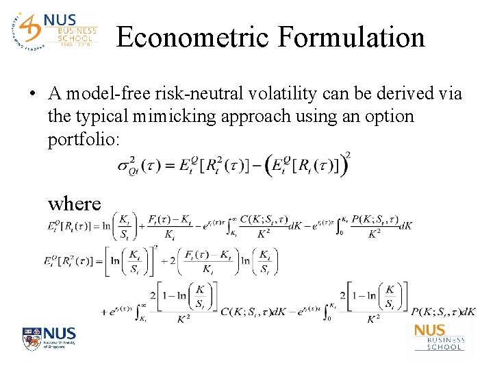
Econometric Formulation • A model-free risk-neutral volatility can be derived via the typical mimicking approach using an option portfolio: where

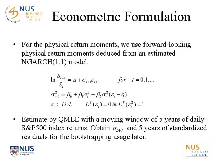
Econometric Formulation • For the physical return moments, we use forward-looking physical return moments deduced from an estimated NGARCH(1, 1) model. • Estimate by QMLE with a moving window of 5 years of daily S&P 500 index returns. Obtain σt+1 and 5 years of standardized residuals for the bootstrapping usage later.

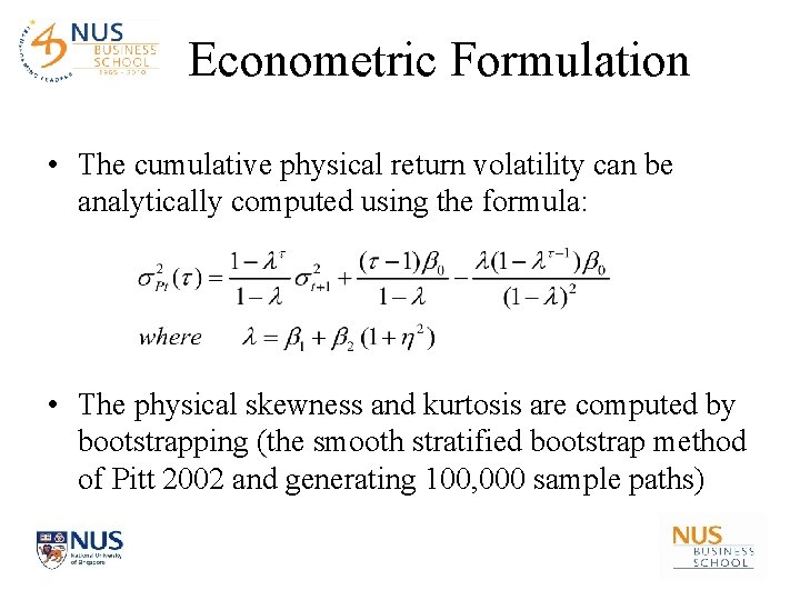
Econometric Formulation • The cumulative physical return volatility can be analytically computed using the formula: • The physical skewness and kurtosis are computed by bootstrapping (the smooth stratified bootstrap method of Pitt 2002 and generating 100, 000 sample paths)

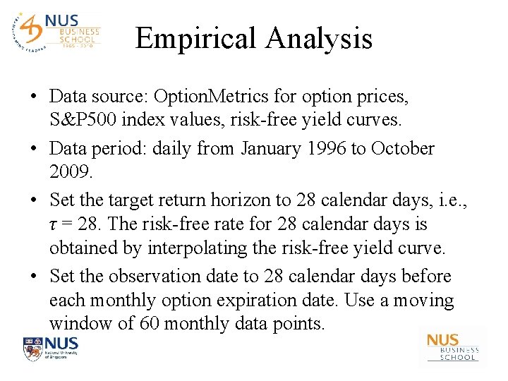
Empirical Analysis • Data source: Option. Metrics for option prices, S&P 500 index values, risk-free yield curves. • Data period: daily from January 1996 to October 2009. • Set the target return horizon to 28 calendar days, i. e. , τ = 28. The risk-free rate for 28 calendar days is obtained by interpolating the risk-free yield curve. • Set the observation date to 28 calendar days before each monthly option expiration date. Use a moving window of 60 monthly data points.

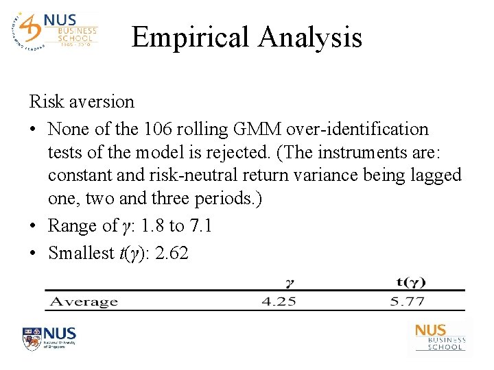
Empirical Analysis Risk aversion • None of the 106 rolling GMM over-identification tests of the model is rejected. (The instruments are: constant and risk-neutral return variance being lagged one, two and three periods. ) • Range of γ: 1. 8 to 7. 1 • Smallest t(γ): 2. 62

Empirical Analysis

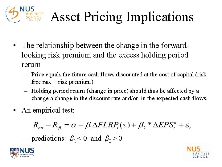
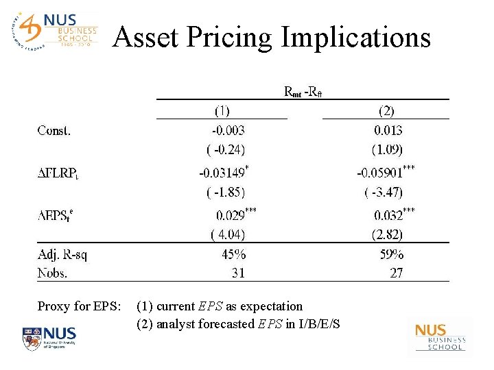
Asset Pricing Implications • The relationship between the change in the forwardlooking risk premium and the excess holding period return – Price equals the future cash flows discounted at the cost of capital (risk free rate + risk premium). – Holding period return (change in price) should thus be affected by a change in the discount rate and/or in the expected cash flows. • An empirical test: – predictions: β 1 < 0 and β 2 > 0.

Asset Pricing Implications Proxy for EPS: (1) current EPS as expectation (2) analyst forecasted EPS in I/B/E/S

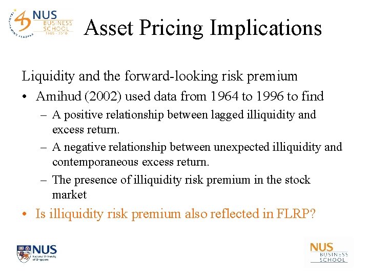
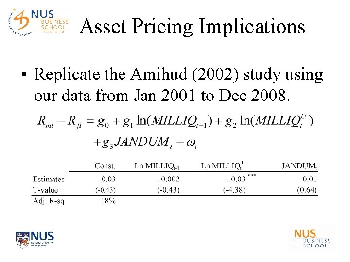
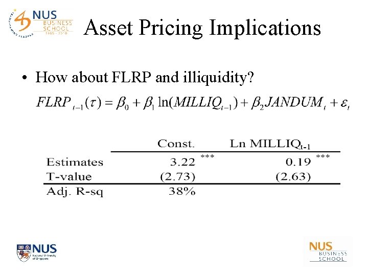
Asset Pricing Implications Liquidity and the forward-looking risk premium • Amihud (2002) used data from 1964 to 1996 to find – A positive relationship between lagged illiquidity and excess return. – A negative relationship between unexpected illiquidity and contemporaneous excess return. – The presence of illiquidity risk premium in the stock market • Is illiquidity risk premium also reflected in FLRP?

Asset Pricing Implications • Replicate the Amihud (2002) study using our data from Jan 2001 to Dec 2008.

Asset Pricing Implications • How about FLRP and illiquidity?

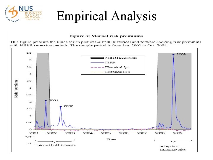
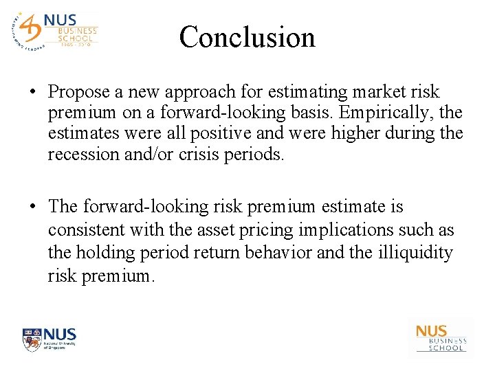
Conclusion • Propose a new approach for estimating market risk premium on a forward-looking basis. Empirically, the estimates were all positive and were higher during the recession and/or crisis periods. • The forward-looking risk premium estimate is consistent with the asset pricing implications such as the holding period return behavior and the illiquidity risk premium.