Forecasting Models3 et Method A 2 1 5

- Slides: 15

Forecasting Models-3

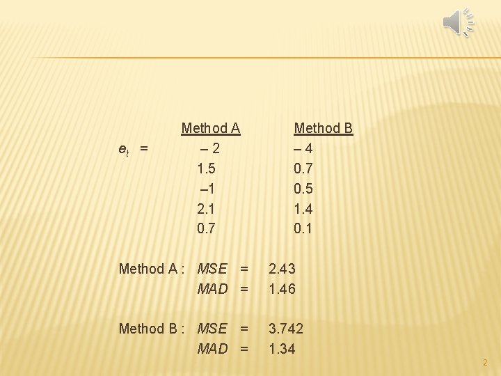
et = Method A – 2 1. 5 – 1 2. 1 0. 7 Method B – 4 0. 7 0. 5 1. 4 0. 1 Method A : MSE = MAD = 2. 43 1. 46 Method B : MSE = MAD = 3. 742 1. 34 2

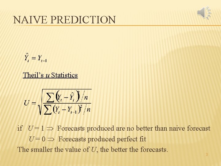
NAIVE PREDICTION Theil’s u Statistics if U = 1 Forecasts produced are no better than naive forecast U = 0 Forecasts produced perfect fit The smaller the value of U, the better the forecasts. 3

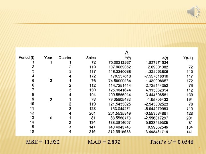
MSE = 11. 932 MAD = 2. 892 Theil’s U = 0. 0546 4

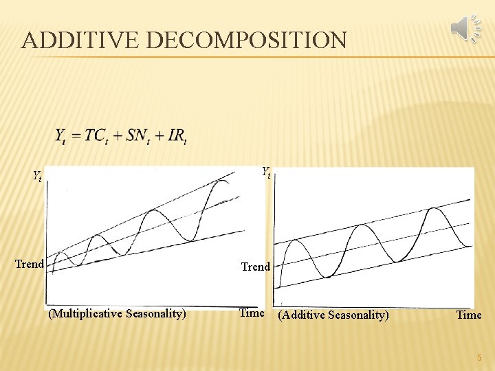
ADDITIVE DECOMPOSITION Yt Yt Trend (Multiplicative Seasonality) Time (Additive Seasonality) Time 5

CAUSAL FORECASTING MODELS � Forecasting a dependent variable based on other (independent) variables � Uses simple or multiple regression � Example: � Dependent variable: Swimwear sales � Independent variables: selling price, competitors prices, temperature, advertising

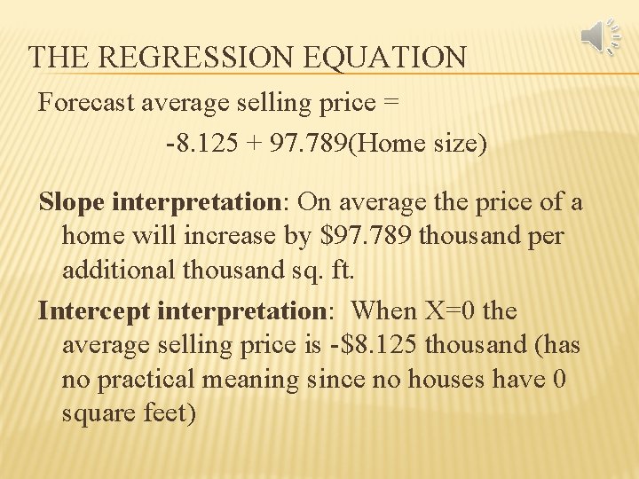
THE REGRESSION EQUATION Forecast average selling price = -8. 125 + 97. 789(Home size) Slope interpretation: On average the price of a home will increase by $97. 789 thousand per additional thousand sq. ft. Intercept interpretation: When X=0 the average selling price is -$8. 125 thousand (has no practical meaning since no houses have 0 square feet)

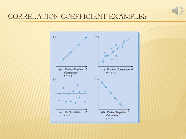
STANDARD ERROR AND CORRELATION � Standard Error (Sy, x) – the standard deviation of the regression equation (useful for confidence intervals on forecasts) � Correlation Coefficient (r) – measures the strength of the linear relation -1 < r < 1

CORRELATION COEFFICIENT EXAMPLES

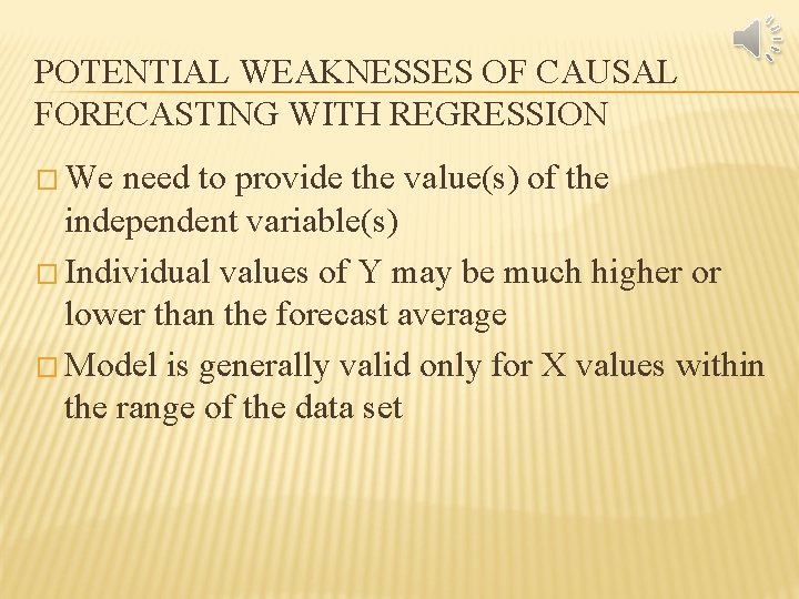
POTENTIAL WEAKNESSES OF CAUSAL FORECASTING WITH REGRESSION � We need to provide the value(s) of the independent variable(s) � Individual values of Y may be much higher or lower than the forecast average � Model is generally valid only for X values within the range of the data set

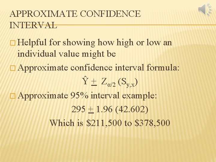
APPROXIMATE CONFIDENCE INTERVAL � Helpful for showing how high or low an individual value might be � Approximate confidence interval formula: Ŷ + Zα/2 (Sy, x) � Approximate 95% interval example: 295 + 1. 96 (42. 602) Which is $211, 500 to $378, 500

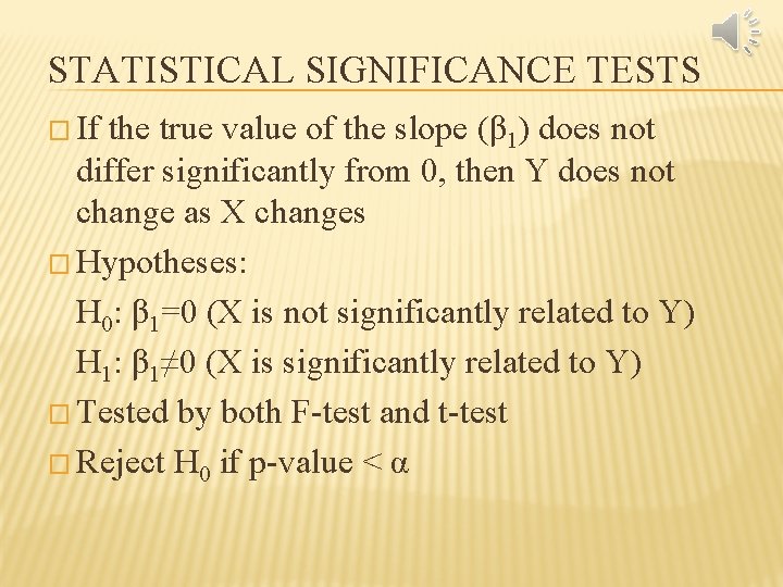
STATISTICAL SIGNIFICANCE TESTS � If the true value of the slope (β 1) does not differ significantly from 0, then Y does not change as X changes � Hypotheses: H 0: β 1=0 (X is not significantly related to Y) H 1: β 1≠ 0 (X is significantly related to Y) � Tested by both F-test and t-test � Reject H 0 if p-value < α

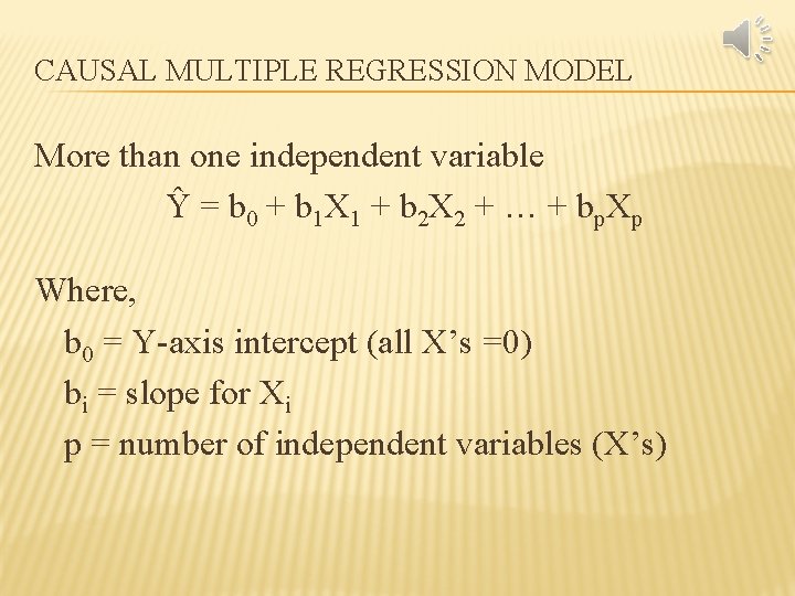
CAUSAL MULTIPLE REGRESSION MODEL More than one independent variable Ŷ = b 0 + b 1 X 1 + b 2 X 2 + … + bp. Xp Where, b 0 = Y-axis intercept (all X’s =0) bi = slope for Xi p = number of independent variables (X’s)

HYPOTHESIS TEST RESULTS FOR HOME SELLING PRICES � F-test: Overall model has significant ability to predict home prices � T-tests: Land area – is significant, given the presence of home size Home size – is not significant, given the presence of land area

MULTICOLLINEARITY � Why did home size become nonsignificant when land area was added? � Multicollinearity exists when 2 or more independent variables are highly correlated � Correlations among X’s can be used to detect multicollinearity