Flow Fields Hao Li and Howard Hamilton Motivation

Flow Fields Hao Li and Howard Hamilton

Motivation for Flow Fields l Multiple AI algorithms in a computer game can produce conflicting results. The AI must resolve these conflicts and find a simultaneous solution.

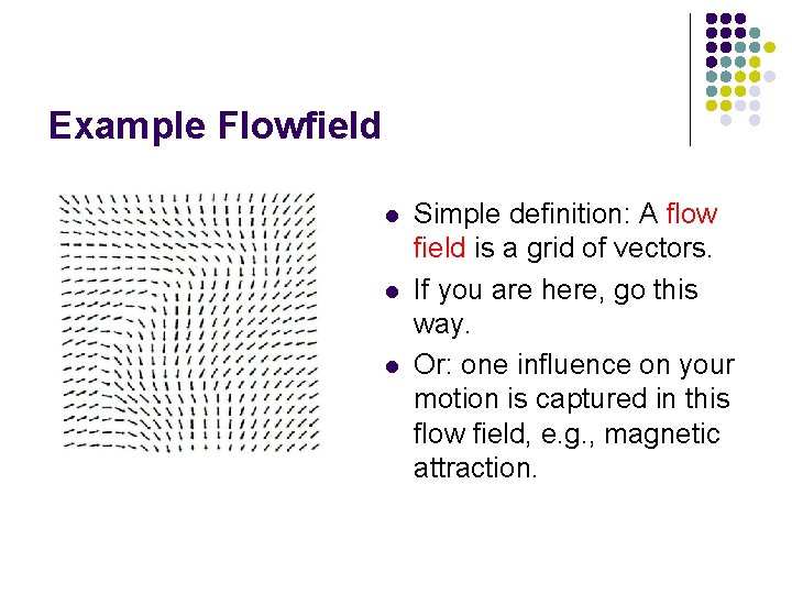
Example Flowfield l l l Simple definition: A flow field is a grid of vectors. If you are here, go this way. Or: one influence on your motion is captured in this flow field, e. g. , magnetic attraction.

Flow Field l l “A flow field consists of a three-dimensional sample space that returns a vector at every point, indicating an attraction toward objects of interest or repulsion away from objects to be avoided” [Alexander, 2006]. We will concentrate on two-dimensional flow fields.

A flow field has two components: l A static data set constructed around static objects (e. g. terrain) l A dynamically generated data set constructed around dynamic objects (e. g. vehicles)

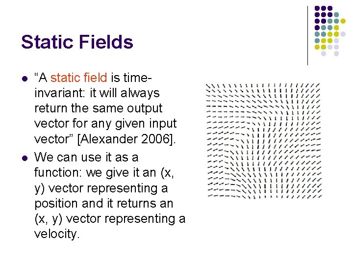
Static Fields l l “A static field is timeinvariant: it will always return the same output vector for any given input vector” [Alexander 2006]. We can use it as a function: we give it an (x, y) vector representing a position and it returns an (x, y) vector representing a velocity.

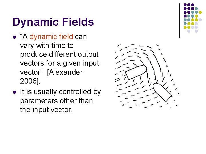
Dynamic Fields l l “A dynamic field can vary with time to produce different output vectors for a given input vector” [Alexander 2006]. It is usually controlled by parameters other than the input vector.

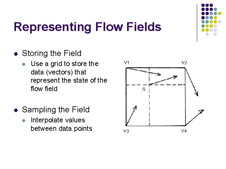
Representing Flow Fields l Storing the Field l l Use a grid to store the data (vectors) that represent the state of the flow field Sampling the Field l Interpolate values between data points

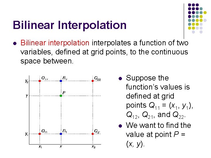
Bilinear Interpolation l Bilinear interpolation interpolates a function of two variables, defined at grid points, to the continuous space between. l l Suppose the function’s values is defined at grid points Q 11 = (x 1, y 1), Q 12, Q 21, and Q 22. We want to find the value at point P = (x, y).

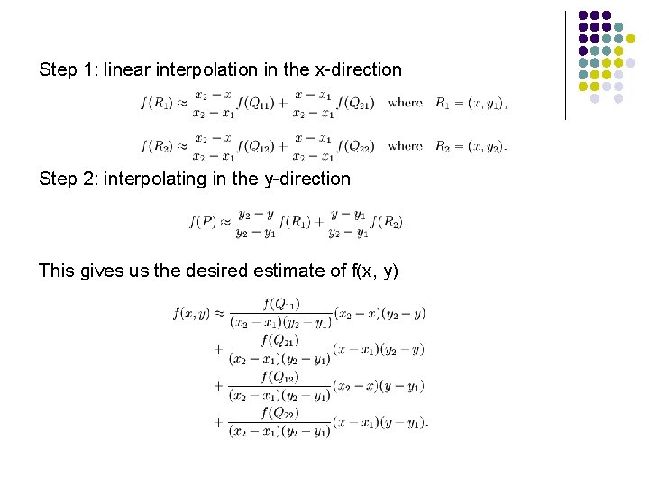
Step 1: linear interpolation in the x-direction Step 2: interpolating in the y-direction This gives us the desired estimate of f(x, y)

Combining Fields l Weighted Addition (+) Take all of the component fields into account and provide the ability to prioritize some fields. l Conditional Operation (OR) Allow one field to completely override other fields. l Field Multiplication (*) Scaling value for each point in the field is the result of sampling another field. (Scaling or dot product)

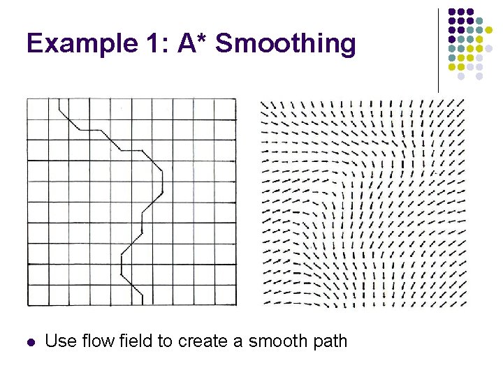
Example 1: A* Smoothing l Use flow field to create a smooth path

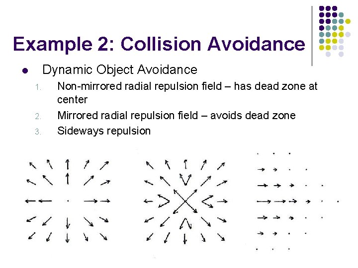
Example 2: Collision Avoidance Dynamic Object Avoidance l 1. 2. 3. Non-mirrored radial repulsion field – has dead zone at center Mirrored radial repulsion field – avoids dead zone Sideways repulsion

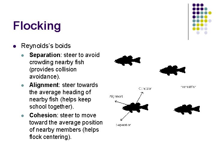
Flocking l Reynolds’s boids l l l Separation: steer to avoid crowding nearby fish (provides collision avoidance). Alignment: steer towards the average heading of nearby fish (helps keep school together). Cohesion: steer to move toward the average position of nearby members (helps flock centering).

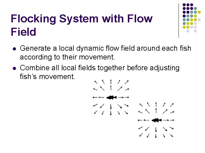
Flocking System with Flow Field l l Generate a local dynamic flow field around each fish according to their movement. Combine all local fields together before adjusting fish’s movement.

Sources of Flow Fields l l l Visualization and editing tools can be used to create flow fields. Convert from a 2 -D sample to a 3 -D sample. Brushes can be used to create a good flow field.

Conclusion l l Flow fields provide elegant solutions to a wide variety of problems. They greatly reduce problems such as oscillation by representing smooth flow rather than giving different results at nearby samples.