Economic Geography 6 Location of industrial activities 121

Economic Geography 6 – Location of industrial activities 121 EC A. Y. 2017/2018 Dr. Giuseppe Borruso Department of Economics, Business, Mathematics and Statistics University of Trieste E-mail. giuseppe. borruso@econ. units. it Ph. +39 040 558 7008 Skype: giuseppe. borruso

Industrial location theory Weber’s model

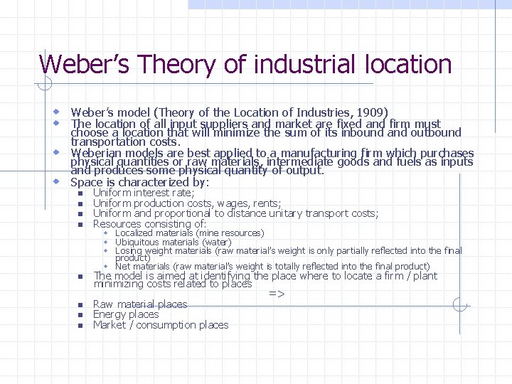
Weber’s Theory of industrial location w Weber’s model (Theory of the Location of Industries, 1909) w The location of all input suppliers and market are fixed and firm must choose a location that will minimize the sum of its inbound and outbound transportation costs. w Weberian models are best applied to a manufacturing firm which purchases physical quantities or raw materials, intermediate goods and fuels as inputs and produces some physical quantity of output. w Space is characterized by: n n n n Uniform interest rate; Uniform production costs, wages, rents; Uniform and proportional to distance unitary transport costs; Resources consisting of: w Localized materials (mine resources) w Ubiquitous materials (water) w Losing weight materials (raw material’s weight is only partially reflected into the final product) w Net materials (raw material’s weight is totally reflected into the final product) The model is aimed at identifying the place where to locate a firm / plant minimizing costs related to places => Raw material places Energy places Market / consumption places

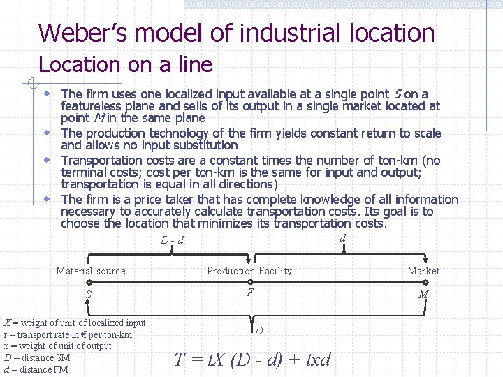
Weber’s model of industrial location Location on a line w The firm uses one localized input available at a single point S on a featureless plane and sells of its output in a single market located at point M in the same plane w The production technology of the firm yields constant return to scale and allows no input substitution w Transportation costs are a constant times the number of ton-km (no terminal costs; cost per ton-km is the same for input and output; transportation is equal in all directions) w The firm is a price taker that has complete knowledge of all information necessary to accurately calculate transportation costs. Its goal is to choose the location that minimizes its transportation costs. d D-d Material source Production Facility Market S F M X = weight of unit of localized input t = transport rate in € per ton-km x = weight of unit of output D = distance SM d = distance FM D T = t. X (D - d) + txd

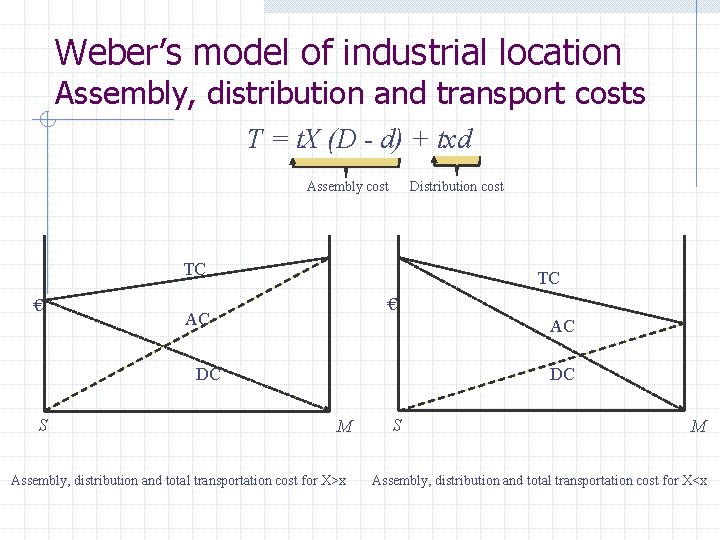
Weber’s model of industrial location Assembly, distribution and transport costs T = t. X (D - d) + txd Assembly cost Distribution cost TC € AC AC DC DC S M Assembly, distribution and total transportation cost for X>x S M Assembly, distribution and total transportation cost for X<x

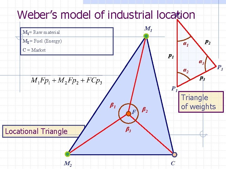
P Weber’s model of industrial location 2 M 1= Raw material M 2 = Fuel (Energy) p 2 α 1 C = Market p 1 α 3 α 2 P 1 β 1 Locational Triangle M 2 F β 2 β 3 C p 3 Triangle of weights P 3

Alternatives: the Varignon Machine w The idea is to take a board and drill holes through all the points. Next, we hang a weight through each hole using a string. We tie all the strings together at one point above the board, and let the system balance itself out. Under unreasonable physical assumptions (i. e. , no friction, etc) the knot will be located at the one median. It is intuitively clear why this is the solution, and a formal proof is easy. Interestingly, this machine was supposedly used in real life to solve the problem in some cases.

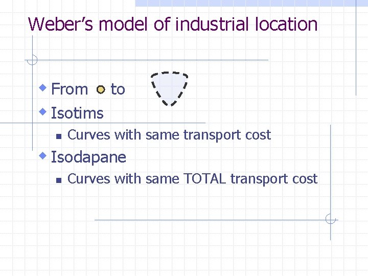
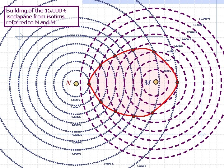
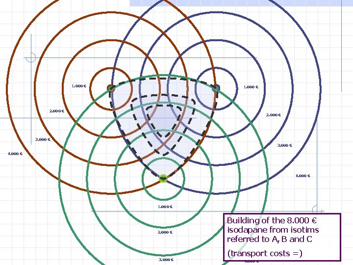
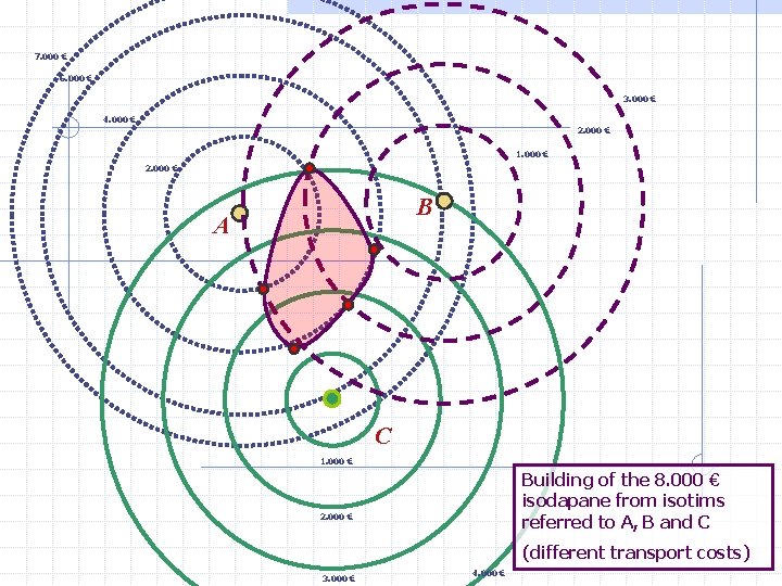
Weber’s model of industrial location w From to w Isotims n Curves with same transport cost w Isodapane n Curves with same TOTAL transport cost

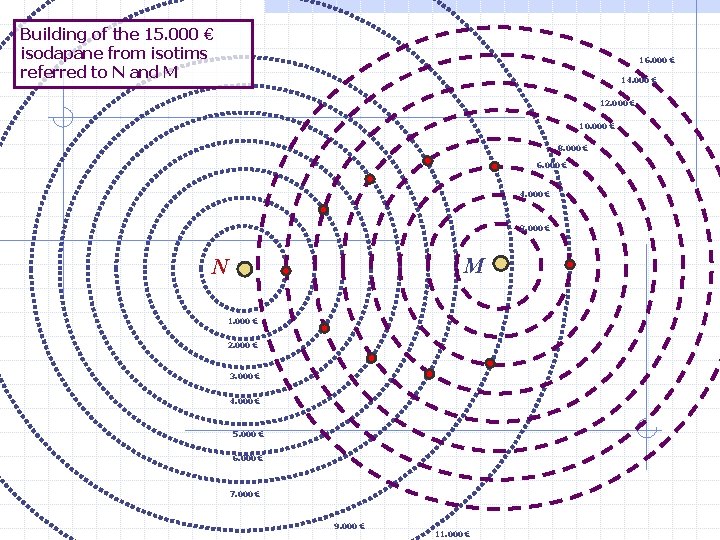
Building of the 15. 000 € isodapane from isotims referred to N and M 16. 000 € 14. 000 € 12. 000 € 10. 000 € 8. 000 € 6. 000 € 4. 000 € 2. 000 € M N 1. 000 € 2. 000 € 3. 000 € 4. 000 € 5. 000 € 6. 000 € 7. 000 € 9. 000 € 11. 000 €

Building of the 15. 000 € isodapane from isotims referred to N and M 16. 000 € 14. 000 € 12. 000 € 10. 000 € 8. 000 € 6. 000 € 4. 000 € 2. 000 € M N 1. 000 € 2. 000 € 3. 000 € 4. 000 € 5. 000 € 6. 000 € 7. 000 € 9. 000 € 11. 000 €

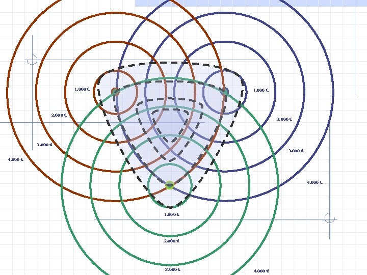
1. 000 € 2. 000 € 3. 000 € 4. 000 € 1. 000 € 2. 000 € 3. 000 € Building of the 8. 000 € isodapane from isotims referred to A, B and C (transport costs =) 4. 000 €

7. 000 € 6. 000 € 3. 000 € 4. 000 € 2. 000 € 1. 000 € 2. 000 € B A C 1. 000 € Building of the 8. 000 € isodapane from isotims referred to A, B and C 2. 000 € (different transport costs) 3. 000 € 4. 000 €

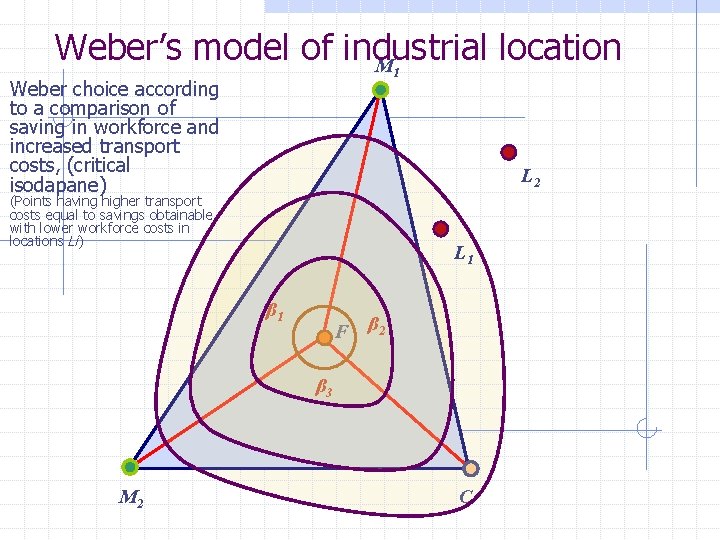
Weber’s model of industrial location M 1 Weber choice according to a comparison of saving in workforce and increased transport costs, (critical isodapane) L 2 (Points having higher transport costs equal to savings obtainable with lower workforce costs in locations Li) L 1 β 1 F β 2 β 3 M 2 C

1. 000 € 2. 000 € 3. 000 € 4. 000 €

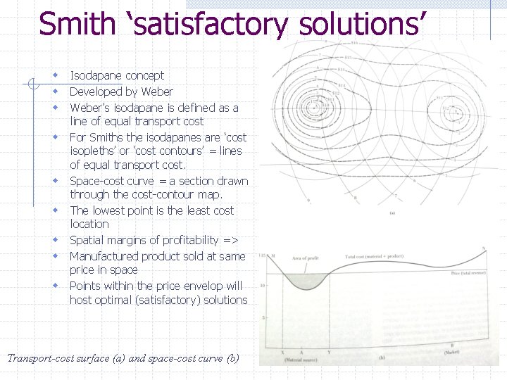
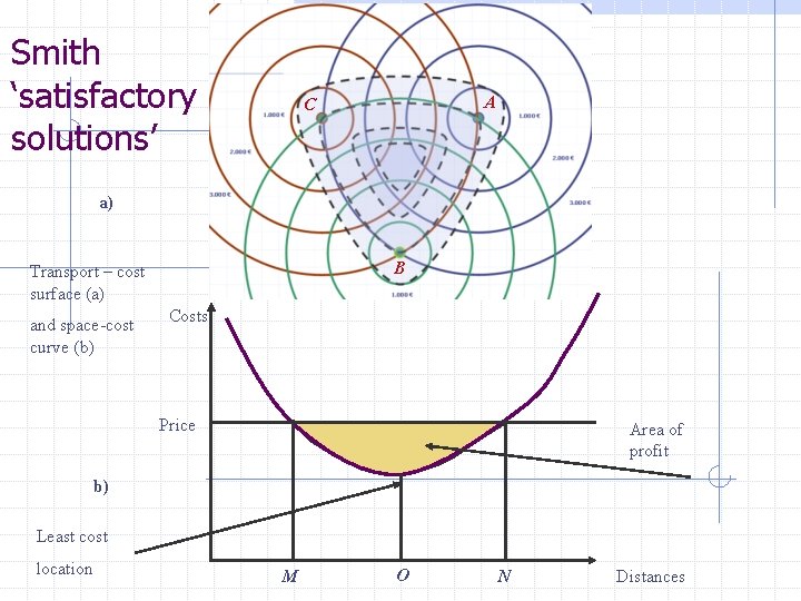
Smith ‘satisfactory solutions’ w Isodapane concept w Developed by Weber w Weber’s isodapane is defined as a w w w line of equal transport cost For Smiths the isodapanes are ‘cost isopleths’ or ‘cost contours’ = lines of equal transport cost. Space-cost curve = a section drawn through the cost-contour map. The lowest point is the least cost location Spatial margins of profitability => Manufactured product sold at same price in space Points within the price envelop will host optimal (satisfactory) solutions Transport-cost surface (a) and space-cost curve (b)

Smith ‘satisfactory solutions’ A C a) B Transport – cost surface (a) and space-cost curve (b) Costs Price Area of profit b) Least cost location M O N Distances

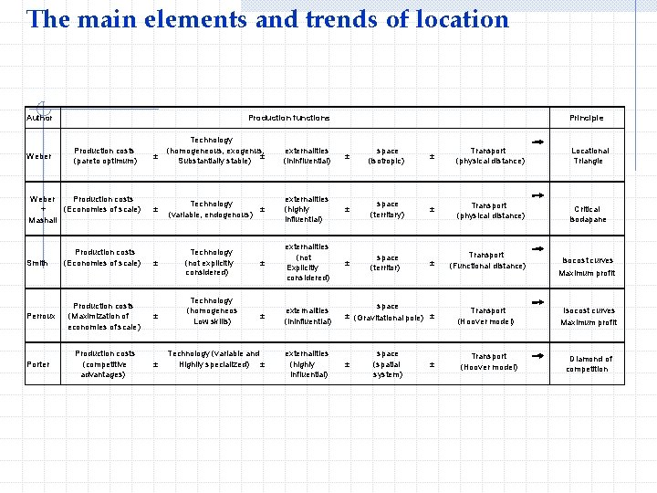
The main elements and trends of location Production functions Author Weber Production costs (pareto optimum) Weber Production costs (Economies of scale) + Mashall Smith Perroux Porter Production costs (Economies of scale) ± ± ± Production costs (Maximization of economies of scale) ± Production costs (competitive advantages) ± Technology (homogeneous, exogenus, ± Substantially stable) Technology ± (variable, endogenous) Technology (not explicitly considered) Technology (homogeneos Low skills) ± ± Technology (variable and Highlly specialized) ± Principle externalities (ininfluential) ± space (isotropic) ± Transport (physical distance) Locational Triangle externalities (highly influential) ± space (territory) ± Transport (physical distance) Critical isodapane externalities (not Explicitly considered) ± space (territor) ± Transport (Functional distance) externalities (ininfluential) externalities (highly influential) space ± (Gravitational pole) ± ± space (spatial system) ± Transport (Hoover model) Isocost curves Maximum profit Diamond of competition

References w w w w CONTI S. , Geografia Economica, Torino, Utet, 1996 Porter, M. 1990. The competitive Advantage of Nations. New York: The Free Press. Porter, M. E. 1998. Clusters and the new economics of competition. Harvard Business Review 76 (6): 77 -90. Porter, M. E. 2000. Location, competition, and economic development: Local clusters in a global economy. Economic Development Quarterly 14 (1): 15 -34. Weber, A. 1929. Theory of the Location of Industries. Trans. Friedrich, C. J. Chicago: University of Chicago Press. Hoover, E. M. 1937. Location Theory and the Shoe and Leather Industries. Cambridge, MA: Harvard University Press. Hoover, E. M. 1948. The Location of Economic Activity. New York: Mc. Graw Hill. Isard, W. , Schooler, E. and Vietoricz, T. 1959. Industrial Complex Analysis and Regional Development. New York: John Wiley. Keeble, D. and Wilkinson, F. (Eds. ) 2000. High-Technology Clusters, Networking and Collective Learning in Europe. Aldershot: Ashgate Krugman, P. 1991. Geography and Trade. Cambridge: MIT Press. Krugman, P. 1995. Development, geography, and economic theory. Cambridge: MIT Press. Krugman, P. and Venables, A. J. 1996. Integration, specialization, and adjustment. European Economic Review 40 (3 -5): 959 -967. Marshall, A. 1890. Principles of Economics. London: Macmillan.