Dynamical Downscaling of NASAGISS Model E Using WRF

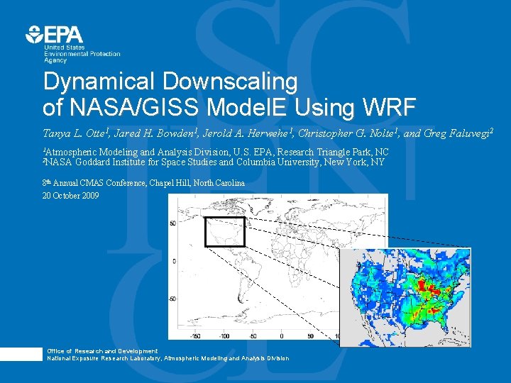
Dynamical Downscaling of NASA/GISS Model. E Using WRF Tanya L. Otte 1, Jared H. Bowden 1, Jerold A. Herwehe 1, Christopher G. Nolte 1, and Greg Faluvegi 2 1 Atmospheric 2 NASA Modeling and Analysis Division, U. S. EPA, Research Triangle Park, NC Goddard Institute for Space Studies and Columbia University, New York, NY 8 th Annual CMAS Conference, Chapel Hill, North Carolina 20 October 2009 Photo image area measures 2” H x 6. 93” W and can be masked by a collage strip of one, two or three images. The photo image area is located 3. 19” from left and 3. 81” from top of page. Each image used in collage should be reducedor cropped to a maximum of 2” high, stroked with a 1. 5 pt white frame and positioned edge-to-edge with accompanying images. Office of Research and Development National Exposure Research Laboratory, Atmospheric Modeling and Analysis Division

Motivations • EPA has a need to predict the regional impacts of climate change on water, air, and ecological systems. • Primary focus is on extreme events (e. g. , heat waves, droughts, flooding, stagnation events) and the frequency of such events, in addition to changes in local mean temperatures and precipitation. • Create strong partnerships with external institutions that have established credible research programs in global climate modeling. • Using “dynamical downscaling”, the regional climate simulations must remain true to the climate trends that are projected by the global climate model. – Need to achieve a delicate balance between the amount of constraint in the regional climate simulations given to the Model. E and the freedom of WRF to simulate its own mesoscale features.

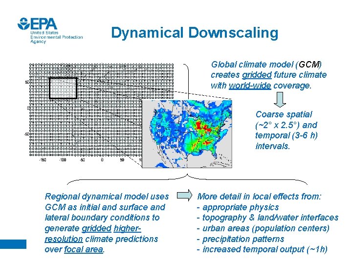
Dynamical Downscaling Global climate model (GCM) creates gridded future climate with world-wide coverage. Coarse spatial (~2° x 2. 5°) and temporal (3 -6 h) intervals. Regional dynamical model uses GCM as initial and surface and lateral boundary conditions to generate gridded higherresolution climate predictions over focal area. More detail in local effects from: - appropriate physics - topography & land/water interfaces - urban areas (population centers) - precipitation patterns - increased temporal output (~1 h)

Approach to Developing Downscaling Methodology • Use reanalysis data as a verifiable surrogate for GCM – Apply reanalysis at GCM’s spatial and temporal resolutions – Validate against observations and/or high-resolution analyses – Similar approach to many other downscaling groups • BUT…also simultaneously developing downscaled fields using GCM output to test downscaling methodology on a parallel track. – Relatively unique approach within regional downscaling community – Allows sanity check of conclusions drawn from reanalysis (i. e. , can we make the “leap of faith” between reanalysis and GCM methods? )

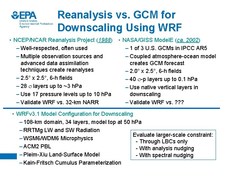
Reanalysis vs. GCM for Downscaling Using WRF • NCEP/NCAR Reanalysis Project (1988) – Well-respected, often used – Multiple observation sources and advanced data assimilation techniques create reanalyses – 2. 5° x 2. 5°, 6 -h fields – 28 s layers up to ~3 h. Pa – Use 17 pressure levels up to 10 h. Pa – Validate WRF vs. 32 -km NARR • NASA/GISS Model. E (ca. 2002) – 1 of 3 U. S. GCMs in IPCC AR 5 – Coupled atmosphere-ocean model creates GCM forecast – 2. 0° x 2. 5°, 6 -h fields – 40 s-p layers up to 0. 1 h. Pa – Use native vertical layers in downscaling – Validate WRF vs. ? ? ? • WRFv 3. 1 Model Configuration for Downscaling – 108 -km domain, 34 layers, model top at 50 h. Pa – RRTMg LW and SW Radiation Evaluate larger-scale constraint: – WSM 6/WDM 6 Microphysics - Through LBCs only – ACM 2 PBL - With analysis nudging – Pleim-Xiu Land-Surface Model - With spectral nudging – Kain-Fritsch Cumulus Parameterization

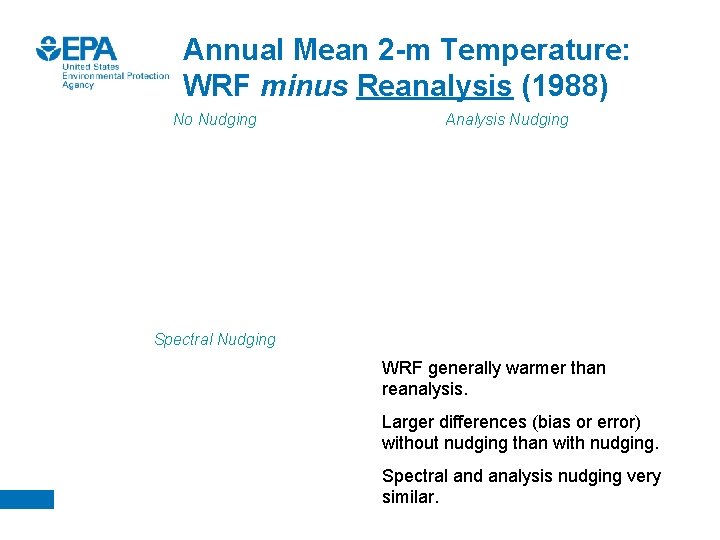
Annual Mean 2 -m Temperature: WRF minus Reanalysis (1988) No Nudging Analysis Nudging Spectral Nudging WRF generally warmer than reanalysis. Larger differences (bias or error) without nudging than with nudging. Spectral and analysis nudging very similar.

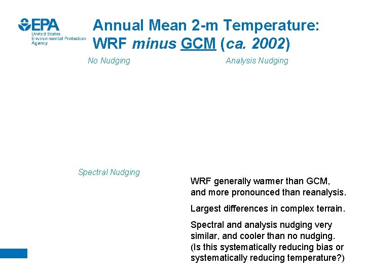
Annual Mean 2 -m Temperature: WRF minus GCM (ca. 2002) No Nudging Spectral Nudging Analysis Nudging WRF generally warmer than GCM, and more pronounced than reanalysis. Largest differences in complex terrain. Spectral and analysis nudging very similar, and cooler than no nudging. (Is this systematically reducing bias or systematically reducing temperature? )

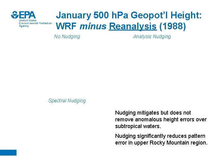
January 500 h. Pa Geopot’l Height: WRF minus Reanalysis (1988) No Nudging Analysis Nudging Spectral Nudging mitigates but does not remove anomalous height errors over subtropical waters. Nudging significantly reduces pattern error in upper Rocky Mountain region.

July 500 h. Pa Geopot’l Height: WRF minus Reanalysis (1988) No Nudging Analysis Nudging Spectral Nudging Larger errors without nudging than with either spectral or analysis nudging. Nudging works to correct pattern errors seen in “no nudging” run. Nudging exacerbates a positive height anomaly in the Plains (lee of Rockies).

A Few Thoughts… • For both reanalysis and GCM, 2 -m temperature differences (i. e. , biases) are lower when either spectral or analysis nudging is used than without nudging. • Differences between WRF simulation and GCM are more pronounced (higher error) than WRF minus reanalysis. – Is this related to higher-resolution detail in WRF than coarse GCM, and, if so, is this adding value? – Or is this related to different behavior of GCM fields than reanalysis in WRF, or different years? – How do we know? How do we relate statistical to physical differences? • Seasonal differences in 2 -m temperature are qualitatively similar to annual differences for both reanalysis and GCM (not shown). • Across the domain, spectral and analysis nudging are qualitatively similar for 2 -m temperature and 500 -h. Pa height under this configuration of WRF. – No clear advantage for either technique yet. – Using either nudging technique is better than no nudging at all.

Daily 2 -m Temperature (1988) Analysis vs. Spectral Nudging: Reanalysis (by region) Regional errors in daily average 2 -m temperature track very closely within each region for analysis and spectral nudging. Changes in weather patterns captured consistently with both methods of nudging. Analysis Nudging Spectral Nudging

Daily Precipitation (1988) Analysis vs. Spectral Nudging: Reanalysis (by region) Regional errors in precipitation reveal seasonal and regional differences in nudging approach. Often errors are more pronounced in summer (convection? ). Larger, widespread differences seen with spectral nudging. At times, analysis nudging has dry bias. Analysis Nudging Spectral Nudging

Daily 2 -m Temperature (ca. 2002) Analysis vs. Spectral Nudging: GCM (by region) Analysis and spectral nudging perform similarly for each region, but more distinction in amplitude than with reanalysis. Regional behavior of bias and magnitude of bias is different with GCM than with reanalysis. Spectral Nudging Analysis Nudging

Daily Precipitation (ca. 2002) Analysis vs. Spectral Nudging: GCM (by region) Larger regional totals with spectral nudging. At times, analysis nudging has dry bias. Magnitude of difference in regional precipitation is much larger with GCM than reanalysis. Significant seasonal differences between nudging methods in the regions Spectral Nudging Analysis Nudging

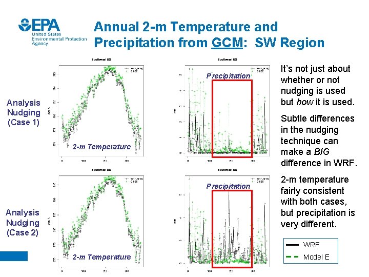
Annual 2 -m Temperature and Precipitation from GCM: SW Region Precipitation Analysis Nudging (Case 1) Subtle differences in the nudging technique can make a BIG difference in WRF. 2 -m Temperature Precipitation Analysis Nudging (Case 2) It’s not just about whether or not nudging is used but how it is used. 2 -m temperature fairly consistent with both cases, but precipitation is very different. WRF 2 -m Temperature Model E

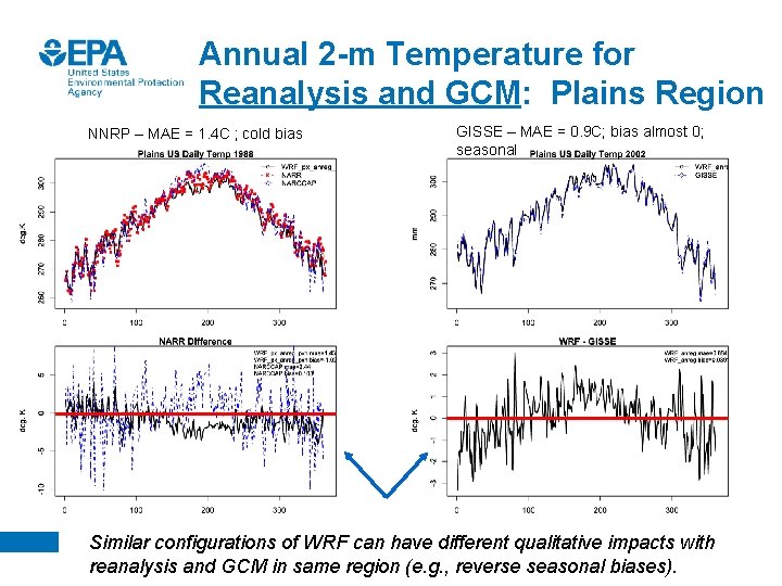
Annual 2 -m Temperature for Reanalysis and GCM: Plains Region NNRP – MAE = 1. 4 C ; cold bias GISSE – MAE = 0. 9 C; bias almost 0; seasonal Similar configurations of WRF can have different qualitative impacts with reanalysis and GCM in same region (e. g. , reverse seasonal biases).

A Few Final Thoughts… • In our testing, RCM simulations are far more sensitive to “nudging vs. no nudging” than changing physics options (not shown). • Both spectral nudging and analysis nudging are improvements over no nudging at all. – Simulations that are only constrained via LBCs rapidly deviate from the larger-scale forcing fields. (Think: “forecast model”. ) – Although spectral nudging is the “hot topic” for regional climate modeling, analysis nudging should not be ignored. – There is little indication of decrease in skill with using nudging over time in an annual simulation. (Could be significant for AQM. ) • Method of nudging (including variables, strength, and where in atmosphere) can have important effects on simulation. • Regional behavior with reanalysis fields (often used to establish downscaling methods) is not necessarily analogous to behavior with GCM fields…at least looking at a single-year simulation. • Near-surface fields (e. g. , 2 -m temperature and precipitation) are easiest to verify, but they do not tell the whole story. Need to look aloft, too!