DifferencesinDifferences Liang Dai Alarm clock again Suppose Alice
- Slides: 15

Differences-in-Differences Liang Dai

Alarm clock again • Suppose Alice starts using alarm clock on June 1. We observe that her average wake-up time in May is 9 am, and that in June is 7 am. • Can we deduce from the time-series difference 7 -9=-2 that alarm clock causes her to wake up earlier? • It could be the case that due to final exams, she would wake up earlier even without alarm

Control group • We need a control group, i. e. , those who never use alarm clocks • Suppose Bob also cares about final exams, but he never uses alarm clocks • In May he wakes up at 8 am, and in June 7 am.

Differences-in-Differences • Event: treatment started in the middle of time range covered by data (in June) for the treated (Alice) • Parallel trend assumption: Assume Bob is a good proxy for Alice HAD she NOT used the alarm. (Think of it as result of randomization) • Then the effect of alarm clock usage of Alice on her wakeup time is: (7 -9)-(7 -8)=-1 • The cross-sectional difference between treated and nontreated in the time series difference • This method allows for unknown factors other than final exams, with unknown impact, as long as they impact treated and non-treated Parallelly absent of treatment, as the impact is cancelled out by cross-sectional differencing

Power of DD • As long as parallel trend assumption holds: – DD allows for selection bias: w/o alarm clocks, Alice wakes up at 9 am while Bob does at 8 am – DD allows for outcome w/o treatment to change over time: exam shorten sleeps for both • Parallel trend assumption is strong: DD per se does not rule out endogeneity problem, as parallel trend assumption may be violated.

Example 1 • Card & Krueger, AER 94 • How do low-wage market employers respond to an increase in minimum wage? • Conventional theory predicts a negative relation. • Event: minimum wage in New Jersey rose from $4. 25 to $5. 05 on April 1, 1992 • Treatment group: fast food restaurants in NJ • Control group: those in east Pennsylvania, right across the Delaware river • Totally 410 stores

• Pre- and Post-event outcomes: employment, prices and wages in Feb and Nov. • Why fast food stores? Low wage; homogeneous skills; good data availability • Justification for Parallel trend assumption: NJ is a small state with an economy closely related to nearby states. • Closed stores are also covered. So survival bias is fixed.

Main results • Employment actually increases with minimum wage (in NJ). Inconsistent with conventional theory • Prices also increase with minimum wage, suggesting pass-through to customers.

Justification against reverse causality • Since regressions are run at store level, it is unlikely that factors concerning a single store could affect minimum wage legislation at state level.

Example 2 • Fisman, AER 01 • Do political connections increase firm value? • Major challenge: other than measurability of connections, ?

Example 2 • Fisman, AER 01 • Do political connections increase firm value? • Major challenge: other than measurability of connections, business acumen is correlated with ability to establish political connections

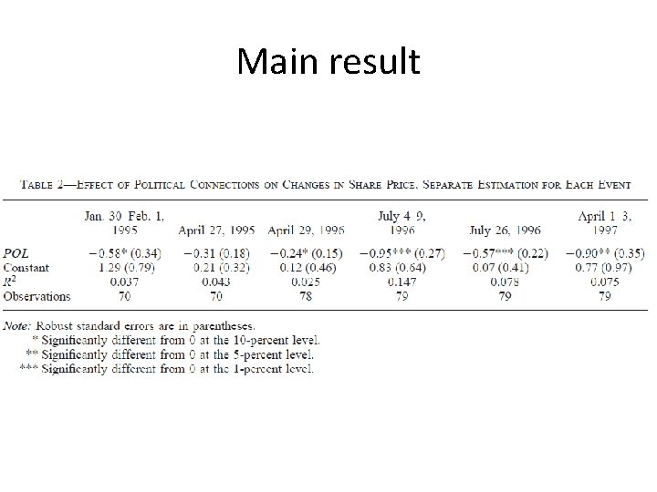
Reversed DD • Context: Indonesia under Suharto reign • Treatment: have political connection with Suharto family and long-term allies • Event: adverse news about Suharto’s health. Connection lost exogenously if he dies • Control group: those without connection to begin with • DD prediction: market value of connected drops by more than unconnected following the news

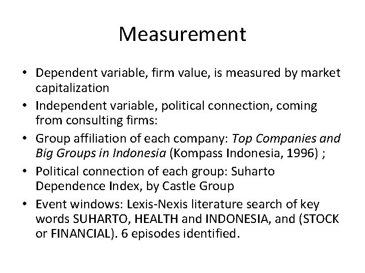
Measurement • Dependent variable, firm value, is measured by market capitalization • Independent variable, political connection, coming from consulting firms: • Group affiliation of each company: Top Companies and Big Groups in Indonesia (Kompass Indonesia, 1996) ; • Political connection of each group: Suharto Dependence Index, by Castle Group • Event windows: Lexis-Nexis literature search of key words SUHARTO, HEALTH and INDONESIA, and (STOCK or FINANCIAL). 6 episodes identified.

Main result

Justification against selection bias • It is unlikely that Suharto’s (unexpected) health problems are driven by decisions of individual firms. • Firms cannot choose to cut the political connection before the news