Deforestation Topdown Modelling Pedro R Andrade Modelling and

Deforestation: Top-down Modelling Pedro R. Andrade

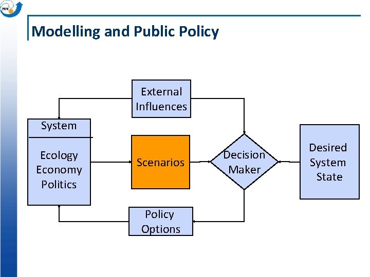
Modelling and Public Policy External Influences System Ecology Economy Politics Scenarios Policy Options Decision Maker Desired System State

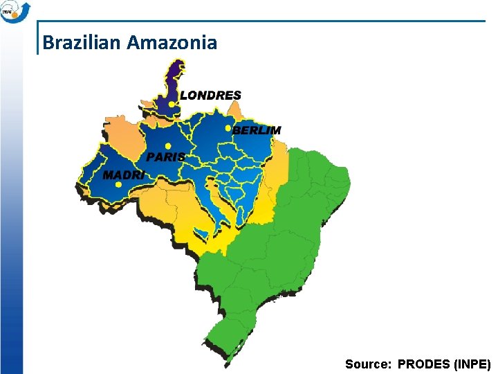
Brazilian Amazonia Source: PRODES (INPE)

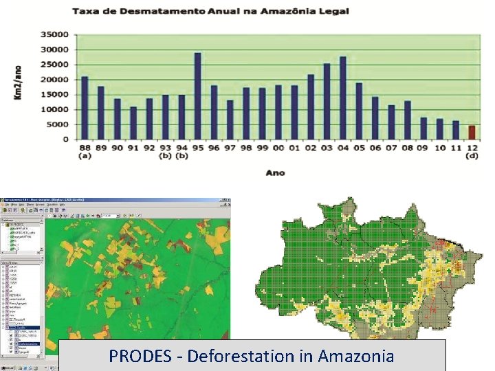
PRODES - Deforestation in Amazonia

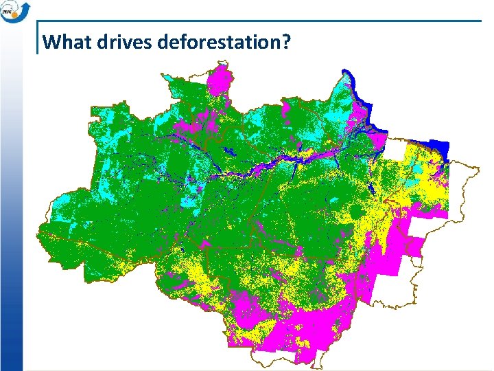
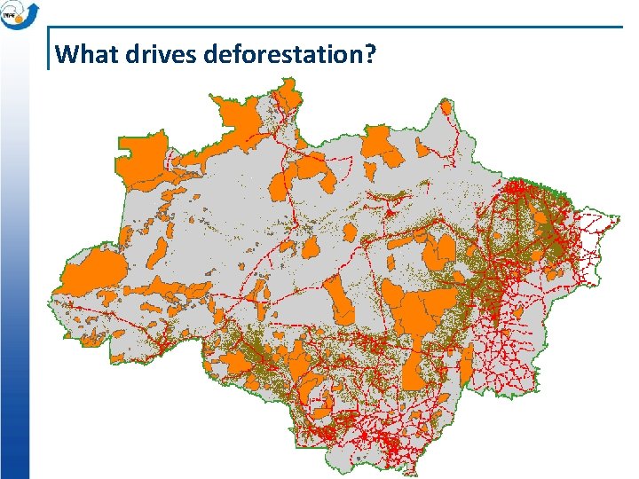
What drives deforestation?

What drives deforestation?

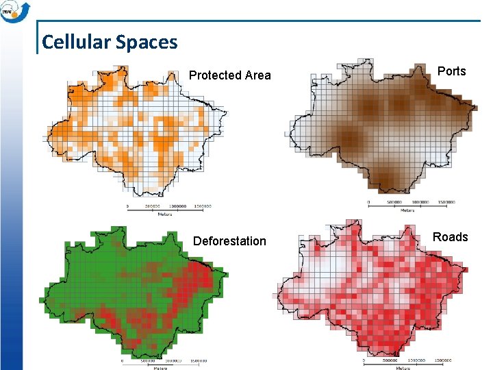
Cellular Spaces Protected Areas Ports Deforestation Roads

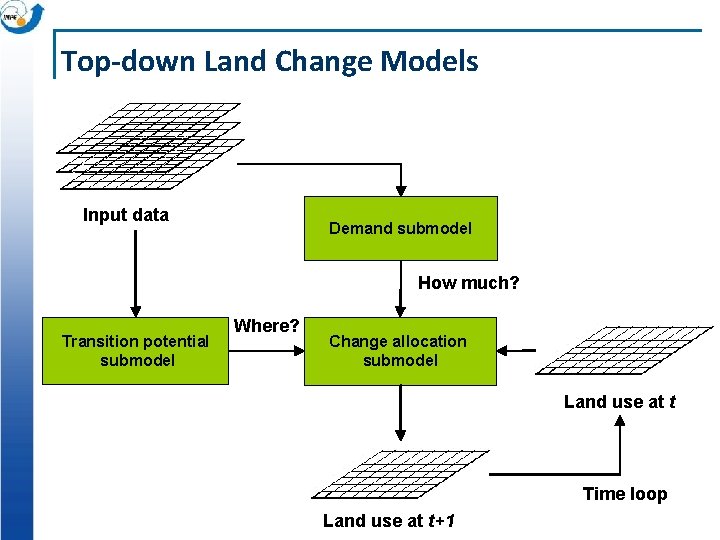
Top-down Land Change Models Input data Demand submodel How much? Transition potential submodel Where? Change allocation submodel Land use at t Time loop Land use at t+1

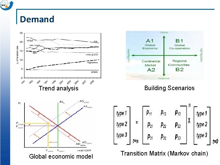
Demand Trend analysis Global economic model Building Scenarios Transition Matrix (Markov chain)

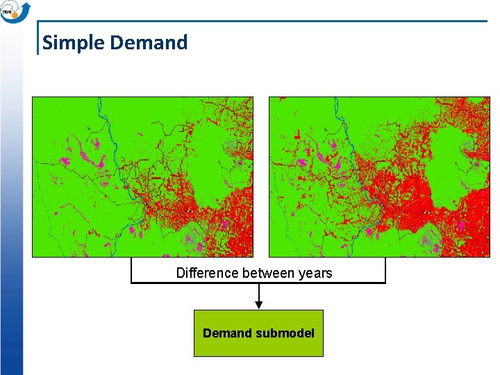
Simple Demand Difference between years Demand submodel

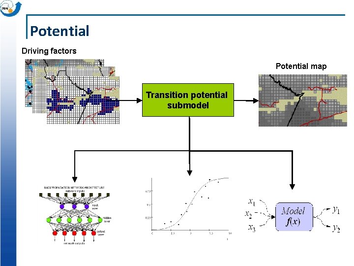
Potential Driving factors Potential map Transition potential submodel Neural Network Multivariate Statistics Mathematics

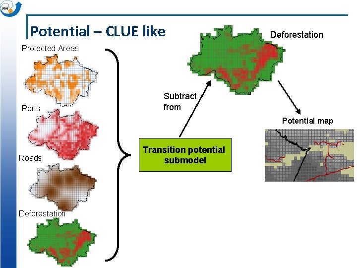
Potential – CLUE like Deforestation Protected Areas Ports Subtract from Potential map Roads Deforestation Transition potential submodel

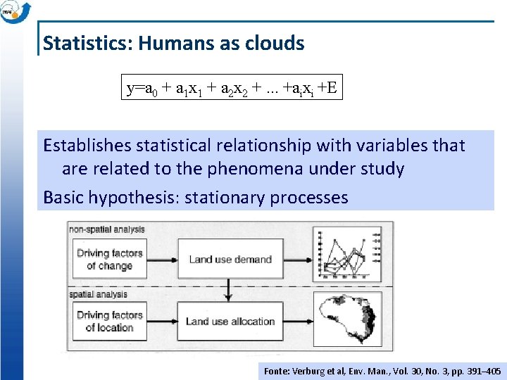
Statistics: Humans as clouds y=a 0 + a 1 x 1 + a 2 x 2 +. . . +aixi +E Establishes statistical relationship with variables that are related to the phenomena under study Basic hypothesis: stationary processes Fonte: Verburg et al, Env. Man. , Vol. 30, No. 3, pp. 391– 405

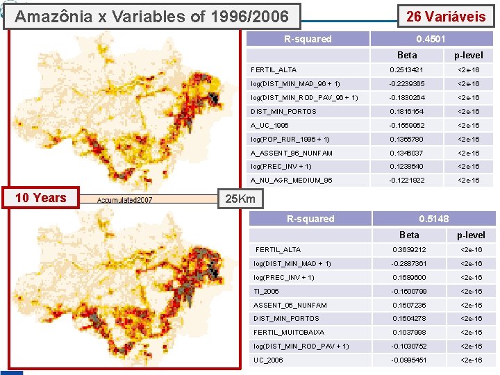
Amazônia x Variables of 1996/2006 26 Variáveis R-squared 10 Years 0. 4501 Beta p-level FERTIL_ALTA 0. 2513421 <2 e-16 log(DIST_MIN_MAD_96 + 1) -0. 2239365 <2 e-16 log(DIST_MIN_ROD_PAV_96 + 1) -0. 1830264 <2 e-16 DIST_MIN_PORTOS 0. 1816154 <2 e-16 A_UC_1996 -0. 1559962 <2 e-16 log(POP_RUR_1996 + 1) 0. 1365780 <2 e-16 A_ASSENT_96_NUNFAM 0. 1346037 <2 e-16 log(PREC_INV + 1) 0. 1238640 <2 e-16 A_NU_AGR_MEDIUM_96 -0. 1221922 <2 e-16 25 Km R-squared 0. 5148 Beta p-level FERTIL_ALTA 0. 3639212 <2 e-16 log(DIST_MIN_MAD + 1) -0. 2887361 <2 e-16 log(PREC_INV + 1) 0. 1689600 <2 e-16 TI_2006 -0. 1600799 <2 e-16 ASSENT_06_NUNFAM 0. 1607236 <2 e-16 DIST_MIN_PORTOS 0. 1604278 <2 e-16 FERTIL_MUITOBAIXA 0. 1037998 <2 e-16 log(DIST_MIN_ROD_PAV + 1) -0. 1030752 <2 e-16 UC_2006 -0. 0995451 <2 e-16

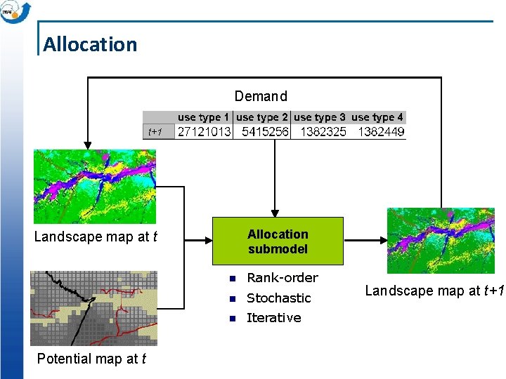
Allocation Demand t+1 Allocation submodel Landscape map at t Potential map at t Rank-order Stochastic Iterative Landscape map at t+1

deforestation. lua Three strategies for computing potential: § Neighborhood: Based on the average deforestation of the neighbors § Regression: Based on distance to roads, ports, and protected areas § Mixed: Based on these four attributes Fixed yearly demand

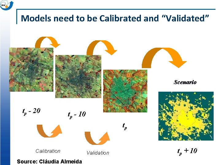
Models need to be Calibrated and “Validated” Scenario tp - 20 tp - 10 tp Calibration Source: Cláudia Almeida Validation tp + 10

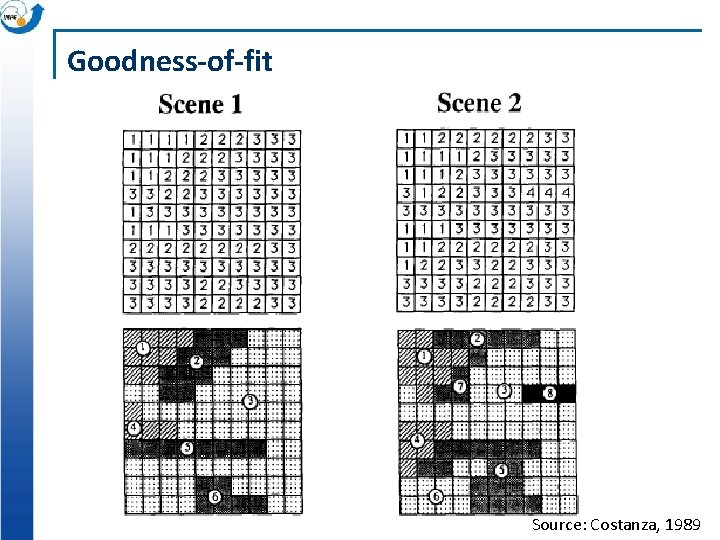
Goodness-of-fit Source: Costanza, 1989

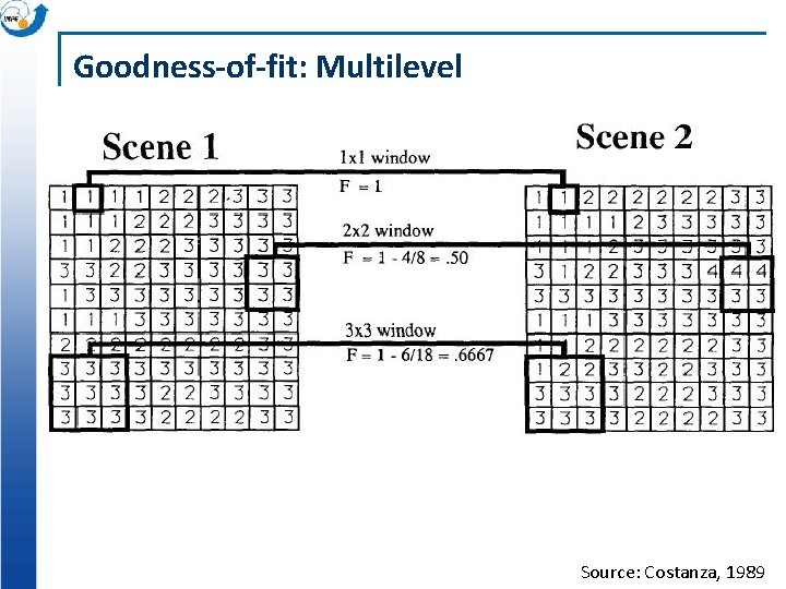
Goodness-of-fit: Multilevel Source: Costanza, 1989

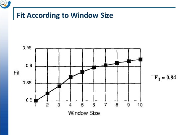
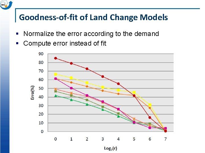
Fit According to Window Size

Goodness-of-fit of Land Change Models § Normalize the error according to the demand § Compute error instead of fit

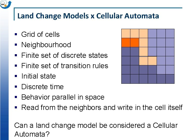
Land Change Models x Cellular Automata § § § § Grid of cells Neighbourhood Finite set of discrete states Finite set of transition rules Initial state Discrete time Behavior parallel in space Read from the neighbors and write in the cell itself Can a land change model be considered a Cellular Automata?