CSC 4170 Theory of Computation Variants of Turing

CSC 4170 Theory of Computation Variants of Turing machines Section 3. 2

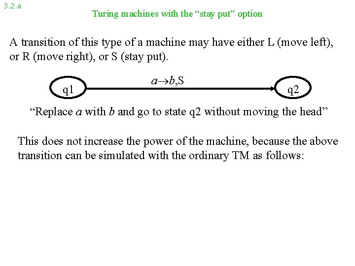
3. 2. a Turing machines with the “stay put” option A transition of this type of a machine may have either L (move left), or R (move right), or S (stay put). q 1 a b, S q 2 “Replace a with b and go to state q 2 without moving the head” This does not increase the power of the machine, because the above transition can be simulated with the ordinary TM as follows:

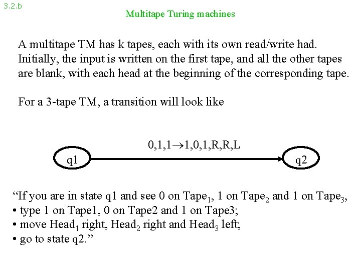
3. 2. b Multitape Turing machines A multitape TM has k tapes, each with its own read/write had. Initially, the input is written on the first tape, and all the other tapes are blank, with each head at the beginning of the corresponding tape. For a 3 -tape TM, a transition will look like 0, 1, 1 1, 0, 1, R, R, L q 1 q 2 “If you are in state q 1 and see 0 on Tape 1, 1 on Tape 2 and 1 on Tape 3, • type 1 on Tape 1, 0 on Tape 2 and 1 on Tape 3; • move Head 1 right, Head 2 right and Head 3 left; • go to state q 2. ”

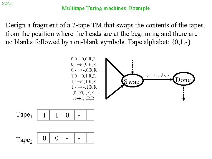
3. 2. c Multitape Turing machines: Example Design a fragment of a 2 -tape TM that swaps the contents of the tapes, from the position where the heads are at the beginning and there are no blanks followed by non-blank symbols. Tape alphabet: {0, 1, -} 0, 0, R, R 0, 1 1, 0, R, R 0, - -, 0, R, R 1, 0 0, 1, R, R 1, - -, 1, R, R -, 0 0, -, R, R -, 1 1, -, R, R Tape 1 1 1 0 - Tape 2 0 0 - - -, - - , -, L, L Swap Done

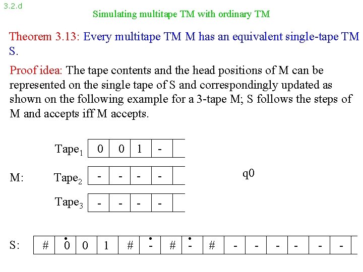
3. 2. d Simulating multitape TM with ordinary TM Theorem 3. 13: Every multitape TM M has an equivalent single-tape TM S. Proof idea: The tape contents and the head positions of M can be represented on the single tape of S and correspondingly updated as shown on the following example for a 3 -tape M; S follows the steps of M and accepts iff M accepts. M: S: # Tape 1 0 0 1 - Tape 2 - - Tape 3 - - . 0 0 1 # . - q 0 # . - # - - -

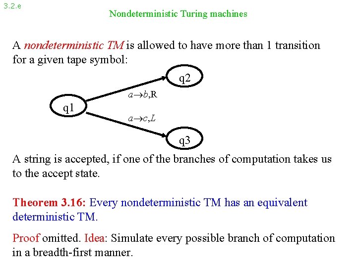
3. 2. e Nondeterministic Turing machines A nondeterministic TM is allowed to have more than 1 transition for a given tape symbol: q 2 a b, R q 1 a c, L q 3 A string is accepted, if one of the branches of computation takes us to the accept state. Theorem 3. 16: Every nondeterministic TM has an equivalent deterministic TM. Proof omitted. Idea: Simulate every possible branch of computation in a breadth-first manner.

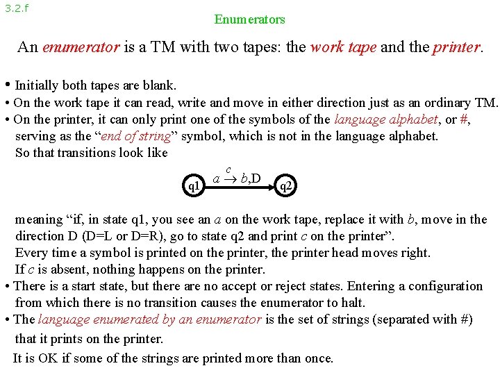
3. 2. f Enumerators An enumerator is a TM with two tapes: the work tape and the printer. • Initially both tapes are blank. • On the work tape it can read, write and move in either direction just as an ordinary TM. • On the printer, it can only print one of the symbols of the language alphabet, or #, serving as the “end of string” symbol, which is not in the language alphabet. So that transitions look like c q 1 a b, D q 2 meaning “if, in state q 1, you see an a on the work tape, replace it with b, move in the direction D (D=L or D=R), go to state q 2 and print c on the printer”. Every time a symbol is printed on the printer, the printer head moves right. If c is absent, nothing happens on the printer. • There is a start state, but there are no accept or reject states. Entering a configuration from which there is no transition causes the enumerator to halt. • The language enumerated by an enumerator is the set of strings (separated with #) that it prints on the printer. It is OK if some of the strings are printed more than once.

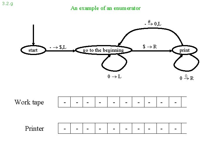
3. 2. g An example of an enumerator # 0, L - start - $, L $ R go to the beginning print 0 L 0 R 0 Work tape - - - - - Printer - - - - -

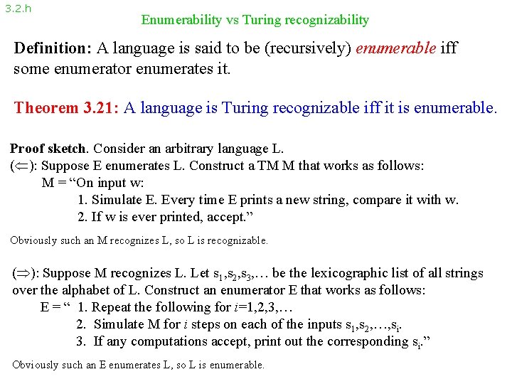
3. 2. h Enumerability vs Turing recognizability Definition: A language is said to be (recursively) enumerable iff some enumerator enumerates it. Theorem 3. 21: A language is Turing recognizable iff it is enumerable. Proof sketch. Consider an arbitrary language L. ( ): Suppose E enumerates L. Construct a TM M that works as follows: M = “On input w: 1. Simulate E. Every time E prints a new string, compare it with w. 2. If w is ever printed, accept. ” Obviously such an M recognizes L, so L is recognizable. ( ): Suppose M recognizes L. Let s 1, s 2, s 3, … be the lexicographic list of all strings over the alphabet of L. Construct an enumerator E that works as follows: E = “ 1. Repeat the following for i=1, 2, 3, … 2. Simulate M for i steps on each of the inputs s 1, s 2, …, si. 3. If any computations accept, print out the corresponding si. ” Obviously such an E enumerates L, so L is enumerable.

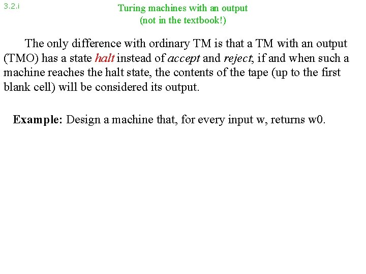
3. 2. i Turing machines with an output (not in the textbook!) The only difference with ordinary TM is that a TM with an output (TMO) has a state halt instead of accept and reject; if and when such a machine reaches the halt state, the contents of the tape (up to the first blank cell) will be considered its output. Example: Design a machine that, for every input w, returns w 0.

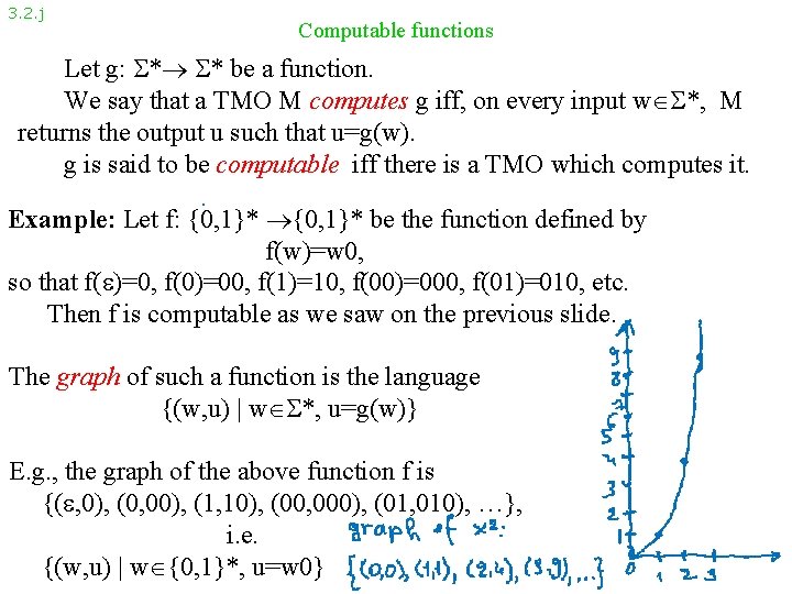
3. 2. j Computable functions Let g: * * be a function. We say that a TMO M computes g iff, on every input w *, M returns the output u such that u=g(w). g is said to be computable iff there is a TMO which computes it. Example: Let f: {0, 1}* be the function defined by f(w)=w 0, so that f( )=0, f(0)=00, f(1)=10, f(00)=000, f(01)=010, etc. Then f is computable as we saw on the previous slide. The graph of such a function is the language {(w, u) | w *, u=g(w)} E. g. , the graph of the above function f is {( , 0), (0, 00), (1, 10), (00, 000), (01, 010), …}, i. e. {(w, u) | w {0, 1}*, u=w 0}

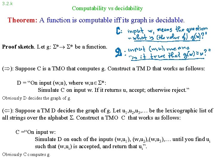
3. 2. k Computability vs decidability Theorem: A function is computable iff its graph is decidable. Proof sketch. Let g: * * be a function. ( ): Suppose C is a TMO that computes g. Construct a TM D that works as follows: D = “On input (w, u), where w, u *: Simulate C on input w. If it returns u, accept; otherwise reject. ” Obviously D decides the graph of g. ( ): Suppose a TM D decides the graph of g. Let u 1, u 2, u 3, … be the lexicographic list of all strings over the alphabet . Construct a TMO C that works as follows: C =“On input w: Simulate D on each of the inputs (w, u 1), (w, u 2), (w, u 3), … until you find ui such that (w, ui) is accepted, and return that ui”. Obviously C computes g.