CREATING MAPS WITH GEOSERVER Accessing geospatial layers in

CREATING MAPS WITH GEOSERVER Accessing geospatial layers in Python and QGIS

What is Geoserver? • Open source solution for sharing geospatial data • Access, share, and publish geospatial layers • Define layer sources once, access them in many formats KML. csv Shapefiles Vector Files GIS Apps Raster Files Geoserver Layers Geo. JSON

Geoserver @ OTN • Layers served out of the OTN Post. GIS database • A few standard public data products available: • Station deployment information (otn: stations, otn: stations_series) • Public animal release information (otn: animals) • Metadata for projects (otn: otn_resources_metadata_points) • Potential to create private per-project layers for HQP use. • Today: two ways to query the OTN Geoserver • code-based (Python) • GUI-based (QGIS)

Querying Geoserver using Python: • “If you wish to make an apple pie from scratch, you must first invent the universe. ” – Carl Sagan • What we’ll need: • Python (2. 7 or better) • The following packages: • numpy, matplotlib, geojson, owslib, cartopy • Optionally • A nice Interactive Development Environment to work in. • Spyder (free) • Py. Charm (cheap and worth it!)

Accessing Geoserver using owslib • Many services available via Geoserver • Shape and point data – Web Feature Service • Rather under-documented at the moment: • To connect to a Geoserver that is implementing WFS: • from owslib. wfs import Web. Feature. Service • wfs = Web. Feature. Service(url, version=“ 2. 0. 0”) • OTN Geoserver url = “http: //global. oceantrack. org: 8080/geoserver/wfs? ” • wfs is now a handle to our Geoserver, and we can run queries like: • wfs. contents = a list of all layers served up by Geoserver • wfs. getfeature(typename=[layername], output. Format=format) • Using the results of getfeature requests, we can build geospatial datasets

Python example: owslib_example. py • Simple script to • connect to Geoserver • grab a layer that defines all stations • generate a printable map • Tools: cartopy, matplotlib, geojson, owslib • Also used: Natural. Earth shapefiles as retrieved by cartopy • naturalearthdata. com

Connecting to Geoserver / getting layers • # Imports to get the data out of Geo. Server from owslib. wfs import Web. Feature. Service import geojson import numpy as np # Imports to plot the data onto a map import cartopy. crs as ccrs import cartopy. feature as feature import matplotlib. pyplot as plt • wfs = Web. Feature. Service('http: //global. oceantrack. org: 8080/geoserver/wfs? ', version="2. 0. 0") • # Print the name of every layer available on this Geoserver print list(wfs. contents) • > [‘discovery_coverage_x_mv’, ‘otn: stations_receivers’, ‘otn: stations’, …] • # Get a list of all stations. Lot of metadata associated with this JSON data. # But for now we're interested in the coordinates. json_response = wfs. getfeature(typename=['otn: stations'], propertyname=None, output. Format='application/json'). read() geom = geojson. loads(json_response) flip_geojson_coordinates(geom) • # geom contains a collection of features, and their default coordinate reference system is a stored property of the collection. print geom['type'], geom['crs'] # check our coordinate reference system > Feature. Collection {u'type': u'EPSG', u'properties': {u'code': u'4326'}}

Geometry object into Cartopy map • ax = plt. axes(projection=ccrs. Plate. Carree()) # Plate. Carree just simplest map projection for this example • # Get a list of all features. locs = geom. get("features", []) • # Each feature has a lot of reference data associated with, as defined in Geoserver. print locs[0]['properties']. keys() > [u'station_type', u'notes', u'locality', u'collectioncode', u'longitude', u'stationclass', u'depth', u'latitude', u'station_name', u'stationstatus' ] • • print locs[0]['properties']. values() > [u'Acoustic', … , u'Cape North to St. Paul Island. ', u'CBS', -60. 33438, u'deployed', 162, 47. 06696, u'CBS 008', u'active'] • # You can subselect here if you need only some of the stations lons, lats = zip(*[(x["geometry"]["coordinates"][0], x["geometry"]["coordinates"][1]) for x in locs if x['properties']['collectioncode']==”HFX"]) • # Do some simple buffering of the map edges based on your returned data. plt. axis([min(lons)-1, max(lons)+1, min(lats)-1, max(lats)+1]) • # Plot the lons and lats, transforming them to the axis projection ax. scatter(lons, lats, transform=ccrs. Plate. Carree(), edgecolors="k", marker='. ’) • ax. stock_img() # fairly nice looking bathymetry provided by Cartopy • # put up some nice looking grid lines gl=ax. gridlines(draw_labels=True) gl. xlabels_top = False gl. ylabels_right = False • # Add the land mass colorings ax. add_feature(feature. Natural. Earth. Feature( 'physical', 'land', '10 m', edgecolor ='face', facecolor=feature. COLORS['land'])) • # You can also define a feature and add it in a separate command states_provinces = feature. Natural. Earth. Feature('cultural', 'admin_1_states_provinces_lines', scale='50 m', facecolor='none') ax. add_feature(states_provinces, edgecolor ='gray’) • # There's also a very simple method to call to draw coastlines on your map. ax. coastlines(resolution="10 m”) • plt. show()

Matplotlib/Cartopy Output

Geoserver data using GIS tools (QGIS) • Lots of tools available to plot data from Geoserver and combine it with data from other sources • Arc. GIS, QGIS, cartodb. com • QGIS is free and open-source, so it will be our example • Download available at: • http: //www. qgis. org • Complete manual online at: • http: //docs. qgis. org/2. 2/en/docs/user_manual/

What we’ll need – using QGIS • Open source tradeoffs: • QGIS is easy to use, but can sometimes be hard to install • Natural. Earth (again, but we’ll get it directly this time) • Grab the Natural. Earth Quickstart pack from naturalearthdata. com • http: //kelso. it/x/nequickstart - includes QGIS and Arc. Map pre-made projects

QGIS – using NE Quickstart’s. qgs • Open Natural_Earth_quick_start_for_QGIS. qgs • Lots of very nice layers pre-styled for you • Can take it as it is, or choose to hide some of the ones you don’t need by deselecting: • 10 m_admin_1_states_provinces • 10 m_urban_areas • etc.

QGIS – using NE Quickstart’s. qgs

Adding our Geoserver to QGIS • Layer - Add WFS Layer • Click New button to add a new source for our WFS layers • Geoserver’s URL a bit different for QGIS: • http: //global. oceantrack. org: 8080/geoserver/ows? version=1. 0. 0& • Username/password not required for public layers • Can provide authorization for private layers here

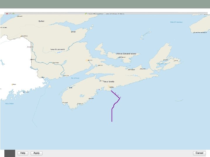
Adding/styling a Geoserver layer • Highlight the layer you want, click Add • The layer appears in your layer list – make sure it’s above the ne_quickstart we added earlier (will be drawn on top) • Double-click to open Layer Properties. Hit Style sub-tab • Change Single Symbol to Categorized • For Column, use ‘collectioncode’ • Hit Classify button • Hit Apply • Stations are grouped and color-coded for you • Further refine station classifications – render certain lines • Can delete all undesired classification groups • Could use rule-based filtering in Style

Adding WFS layer: otn_resources_metadata_points to the map

Tools make everything easier • Now that we have our • • stations, let’s use some detection data Layer – Add Delimited Text Layer Select a Detection Extracts file from the OTN Repository Since this file has Latitude and Longitude, QGIS recognizes its location information and plots it onto a layer All associated data from the file is available to use for filtering/styling/summarizing • Detection Extracts not special, any. csv with lat/lon columns can be ingested this way.

QGIS Print Composer • Lock in a certain style and image layout for printing • Define map areas, inset maps, logos, title graphics, legends • When map layers are updated, legends are repopulated and maps redrawn in-place.

QGIS Print Composer

Geospatial Queries in QGIS • Objects in QGIS are shapes, so intersections between shapes / buffer zones from point data can be queried • Results of that query can be highlighted, eg: • Global coverage • By intersection b/t buffer around station points and coastline shapefile • Add high seas buoys manually afterward

OTN’s Geoserver – for you to use • Geoserver provides layers with data from the OTN DB • Using Python/QGIS, plot formats are reproducible when data is added to the OTN Database • QGIS easier to get started with, and lets you spend more time playing with your data’s style and formatting. • More useful information / learning tools: • Cartopy: http: //scitools. org. uk/cartopy/docs/latest/ • QGIS: http: //www. qgistutorials. com/ • OTN Git. Lab: https: //utility. oceantrack. org/gitlab/