Computational Intelligence Winter Term 201617 Prof Dr Gnter

Computational Intelligence Winter Term 2016/17 Prof. Dr. Günter Rudolph Lehrstuhl für Algorithm Engineering (LS 11) Fakultät für Informatik TU Dortmund

Plan for Today Lecture 04 ● Bidirectional Associative Memory (BAM) § Fixed Points § Concept of Energy Function § Stable States = Minimizers of Energy Function ● Hopfield Network § Convergence § Application to Combinatorial Optimization G. Rudolph: Computational Intelligence ▪ Winter Term 2016/17 2

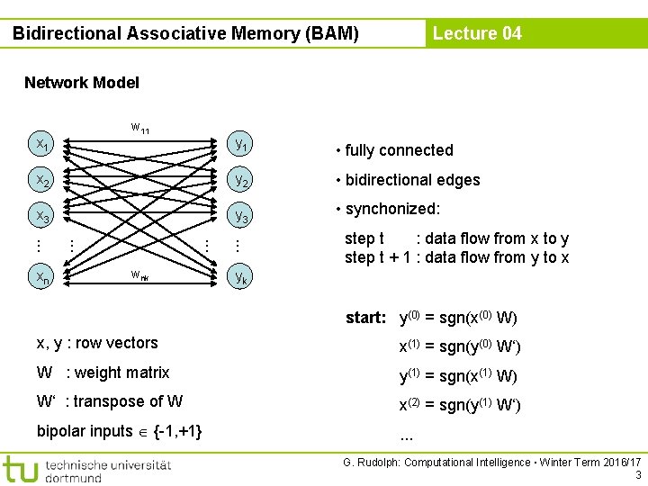
Bidirectional Associative Memory (BAM) Lecture 04 Network Model w 11 x 1 y 1 • fully connected x 2 y 2 • bidirectional edges x 3 y 3 • synchonized: wnk . . . xn step t : data flow from x to y step t + 1 : data flow from y to x yk start: y(0) = sgn(x(0) W) x, y : row vectors x(1) = sgn(y(0) W‘) W : weight matrix y(1) = sgn(x(1) W) W‘ : transpose of W x(2) = sgn(y(1) W‘) bipolar inputs {-1, +1} . . . G. Rudolph: Computational Intelligence ▪ Winter Term 2016/17 3

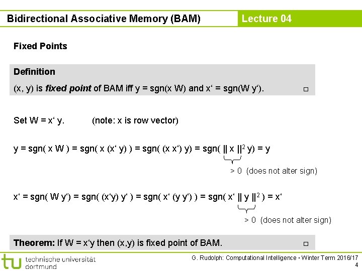
Bidirectional Associative Memory (BAM) Lecture 04 Fixed Points Definition (x, y) is fixed point of BAM iff y = sgn(x W) and x‘ = sgn(W y‘). Set W = x‘ y. □ (note: x is row vector) y = sgn( x W ) = sgn( x (x‘ y) ) = sgn( (x x‘) y) = sgn( || x ||2 y) = y > 0 (does not alter sign) x‘ = sgn( W y‘) = sgn( (x‘y) y‘ ) = sgn( x‘ (y y‘) ) = sgn( x‘ || y ||2 ) = x‘ > 0 (does not alter sign) Theorem: If W = x‘y then (x, y) is fixed point of BAM. □ G. Rudolph: Computational Intelligence ▪ Winter Term 2016/17 4

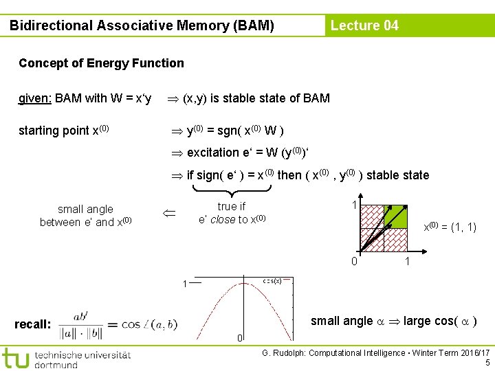
Bidirectional Associative Memory (BAM) Lecture 04 Concept of Energy Function given: BAM with W = x‘y starting point x(0) (x, y) is stable state of BAM y(0) = sgn( x(0) W ) excitation e‘ = W (y(0))‘ if sign( e‘ ) = x(0) then ( x(0) , y(0) ) stable state small angle between e‘ and x(0) true if e‘ close to x(0) 1 x(0) = (1, 1) 0 1 1 small angle large cos( ) recall: 0 G. Rudolph: Computational Intelligence ▪ Winter Term 2016/17 5

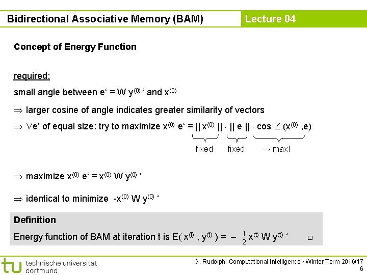
Bidirectional Associative Memory (BAM) Lecture 04 Concept of Energy Function required: small angle between e‘ = W y(0) ‘ and x(0) larger cosine of angle indicates greater similarity of vectors e‘ of equal size: try to maximize x(0) e‘ = || x(0) || ¢ || e || ¢ cos Å (x(0) , e) fixed → max! maximize x(0) e‘ = x(0) W y(0) ‘ identical to minimize -x(0) W y(0) ‘ Definition Energy function of BAM at iteration t is E( x(t) , y(t) ) = – 1 – 2 x(t) W y(t) ‘ □ G. Rudolph: Computational Intelligence ▪ Winter Term 2016/17 6

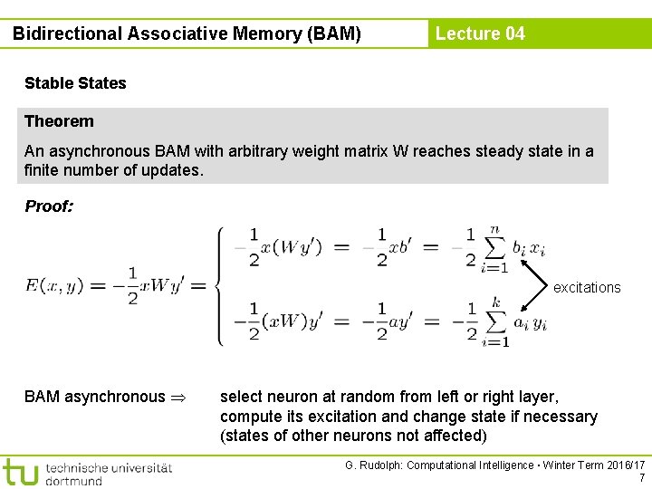
Bidirectional Associative Memory (BAM) Lecture 04 Stable States Theorem An asynchronous BAM with arbitrary weight matrix W reaches steady state in a finite number of updates. Proof: excitations BAM asynchronous select neuron at random from left or right layer, compute its excitation and change state if necessary (states of other neurons not affected) G. Rudolph: Computational Intelligence ▪ Winter Term 2016/17 7

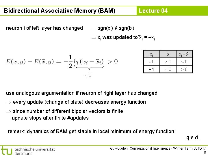
Bidirectional Associative Memory (BAM) neuron i of left layer has changed Lecture 04 sgn(xi) ≠ sgn(bi) xi was updated to ~xi = –xi xi bi xi - ~ xi -1 >0 <0 +1 <0 >0 <0 use analogous argumentation if neuron of right layer has changed every update (change of state) decreases energy function since number of different bipolar vectors is finite update stops after finite #updates remark: dynamics of BAM get stable in local minimum of energy function! q. e. d. G. Rudolph: Computational Intelligence ▪ Winter Term 2016/17 8

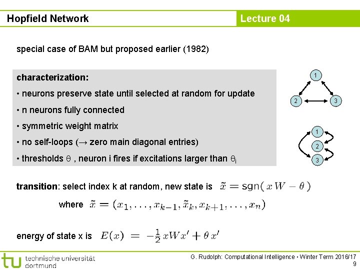
Hopfield Network Lecture 04 special case of BAM but proposed earlier (1982) 1 characterization: • neurons preserve state until selected at random for update 2 3 • n neurons fully connected • symmetric weight matrix 1 • no self-loops (→ zero main diagonal entries) 2 • thresholds , neuron i fires if excitations larger than i 3 transition: select index k at random, new state is where energy of state x is G. Rudolph: Computational Intelligence ▪ Winter Term 2016/17 9

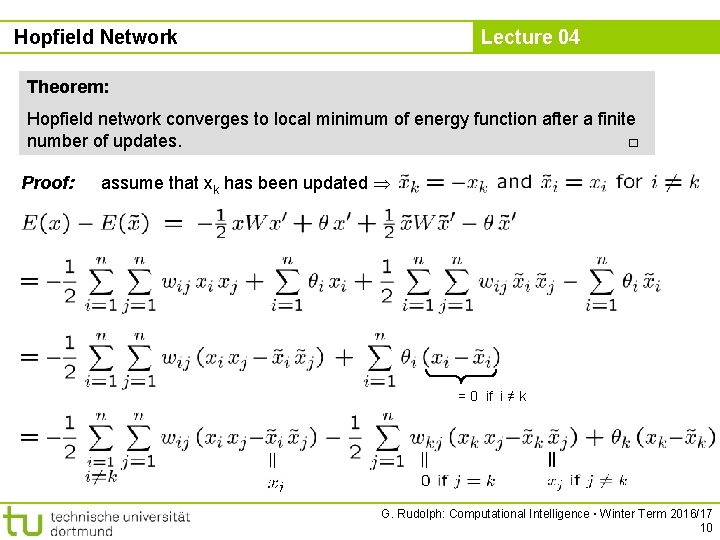
Hopfield Network Lecture 04 Theorem: Hopfield network converges to local minimum of energy function after a finite number of updates. □ Proof: assume that xk has been updated = 0 if i ≠ k G. Rudolph: Computational Intelligence ▪ Winter Term 2016/17 10

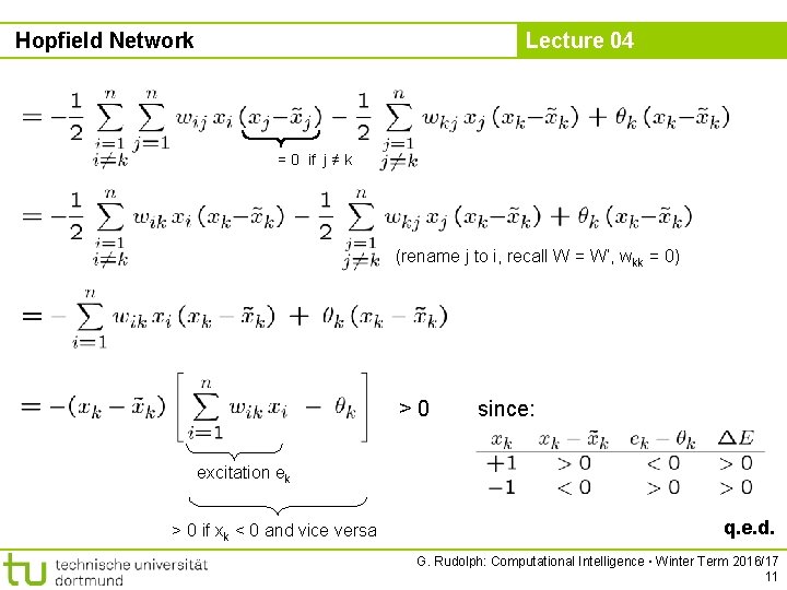
Hopfield Network Lecture 04 = 0 if j ≠ k (rename j to i, recall W = W‘, wkk = 0) >0 since: excitation ek > 0 if xk < 0 and vice versa q. e. d. G. Rudolph: Computational Intelligence ▪ Winter Term 2016/17 11

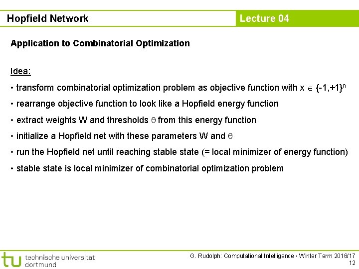
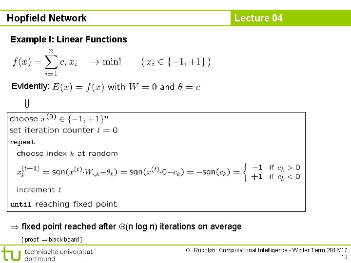
Hopfield Network Lecture 04 Application to Combinatorial Optimization Idea: • transform combinatorial optimization problem as objective function with x {-1, +1}n • rearrange objective function to look like a Hopfield energy function • extract weights W and thresholds from this energy function • initialize a Hopfield net with these parameters W and • run the Hopfield net until reaching stable state (= local minimizer of energy function) • stable state is local minimizer of combinatorial optimization problem G. Rudolph: Computational Intelligence ▪ Winter Term 2016/17 12

Hopfield Network Lecture 04 Example I: Linear Functions Evidently: fixed point reached after (n log n) iterations on average [ proof: → black board ] G. Rudolph: Computational Intelligence ▪ Winter Term 2016/17 13

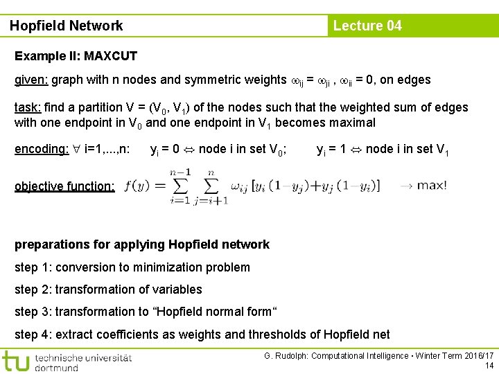
Hopfield Network Lecture 04 Example II: MAXCUT given: graph with n nodes and symmetric weights ij = ji , ii = 0, on edges task: find a partition V = (V 0, V 1) of the nodes such that the weighted sum of edges with one endpoint in V 0 and one endpoint in V 1 becomes maximal encoding: i=1, . . . , n: yi = 0 , node i in set V 0; yi = 1 , node i in set V 1 objective function: preparations for applying Hopfield network step 1: conversion to minimization problem step 2: transformation of variables step 3: transformation to “Hopfield normal form“ step 4: extract coefficients as weights and thresholds of Hopfield net G. Rudolph: Computational Intelligence ▪ Winter Term 2016/17 14

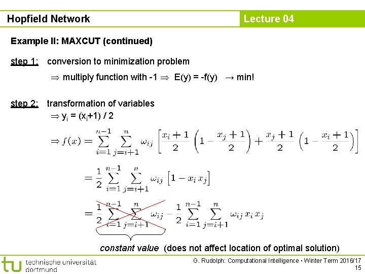
Hopfield Network Lecture 04 Example II: MAXCUT (continued) step 1: conversion to minimization problem multiply function with -1 E(y) = -f(y) → min! step 2: transformation of variables yi = (xi+1) / 2 constant value (does not affect location of optimal solution) G. Rudolph: Computational Intelligence ▪ Winter Term 2016/17 15

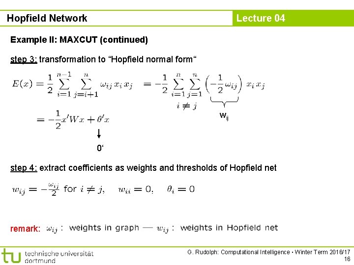
Hopfield Network Lecture 04 Example II: MAXCUT (continued) step 3: transformation to “Hopfield normal form“ wij 0‘ step 4: extract coefficients as weights and thresholds of Hopfield net remark: G. Rudolph: Computational Intelligence ▪ Winter Term 2016/17 16