Computational Intelligence Winter Term 201617 Prof Dr Gnter

Computational Intelligence Winter Term 2016/17 Prof. Dr. Günter Rudolph Lehrstuhl für Algorithm Engineering (LS 11) Fakultät für Informatik TU Dortmund

Plan for Today Lecture 01 Organization (Lectures / Tutorials) Overview CI Introduction to ANN Mc. Culloch Pitts Neuron (MCP) Minsky / Papert Perceptron (MPP) G. Rudolph: Computational Intelligence ▪ Winter Term 2016/17 2

Organizational Issues Lecture 01 Who are you? either studying “Automation and Robotics” (Master of Science) Module “Optimization” or studying “Informatik” - BSc-Modul “Einführung in die Computational Intelligence” - Hauptdiplom-Wahlvorlesung (SPG 6 & 7) or … let me know! G. Rudolph: Computational Intelligence ▪ Winter Term 2016/17 3

Organizational Issues Lecture 01 Who am I ? Günter Rudolph Fakultät für Informatik, LS 11 Guenter. Rudolph@tu-dortmund. de OH-14, R. 232 ← best way to contact me ← if you want to see me office hours: Tuesday, 10: 30– 11: 30 am and by appointment G. Rudolph: Computational Intelligence ▪ Winter Term 2016/17 4

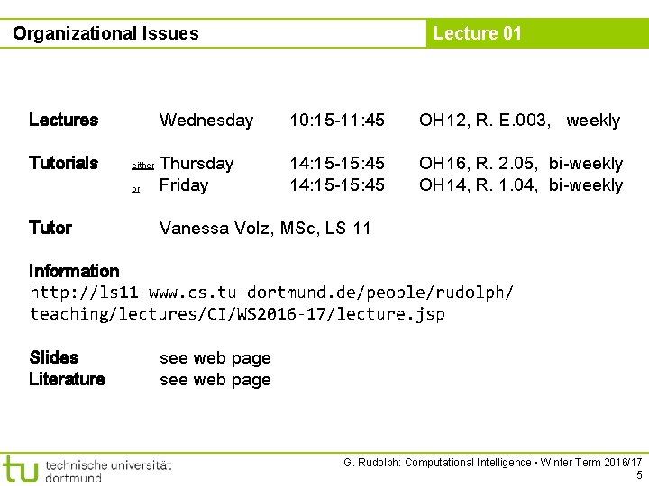
Organizational Issues Lectures Tutorials either or Tutor Lecture 01 Wednesday 10: 15 -11: 45 OH 12, R. E. 003, weekly Thursday Friday 14: 15 -15: 45 OH 16, R. 2. 05, bi-weekly OH 14, R. 1. 04, bi-weekly Vanessa Volz, MSc, LS 11 Information http: //ls 11 -www. cs. tu-dortmund. de/people/rudolph/ teaching/lectures/CI/WS 2016 -17/lecture. jsp Slides Literature see web page G. Rudolph: Computational Intelligence ▪ Winter Term 2016/17 5

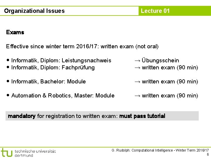
Organizational Issues Lecture 01 Exams Effective since winter term 2016/17: written exam (not oral) ● Informatik, Diplom: Leistungsnachweis ● Informatik, Diplom: Fachprüfung → Übungsschein → written exam (90 min) ● Informatik, Bachelor: Module → written exam (90 min) ● Automation & Robotics, Master: Module → written exam (90 min) mandatory for registration to written exam: must pass tutorial G. Rudolph: Computational Intelligence ▪ Winter Term 2016/17 6

Prerequisites Lecture 01 Knowledge about • mathematics, • programming, • logic is helpful. But what if something is unknown to me? • covered in the lecture • pointers to literature. . . and don‘t hesitate to ask! G. Rudolph: Computational Intelligence ▪ Winter Term 2016/17 7

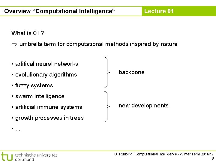
Overview “Computational Intelligence“ Lecture 01 What is CI ? umbrella term for computational methods inspired by nature • artifical neural networks • evolutionary algorithms backbone • fuzzy systems • swarm intelligence • artificial immune systems new developments • growth processes in trees • . . . G. Rudolph: Computational Intelligence ▪ Winter Term 2016/17 8

Overview “Computational Intelligence“ Lecture 01 • term „computational intelligence“ made popular by John Bezdek (FL, USA) • originally intended as a demarcation line establish border between artificial and computational intelligence • nowadays: blurring border our goals: 1. know what CI methods are good for! 2. know when refrain from CI methods! 3. know why they work at all! 4. know how to apply and adjust CI methods to your problem! G. Rudolph: Computational Intelligence ▪ Winter Term 2016/17 9

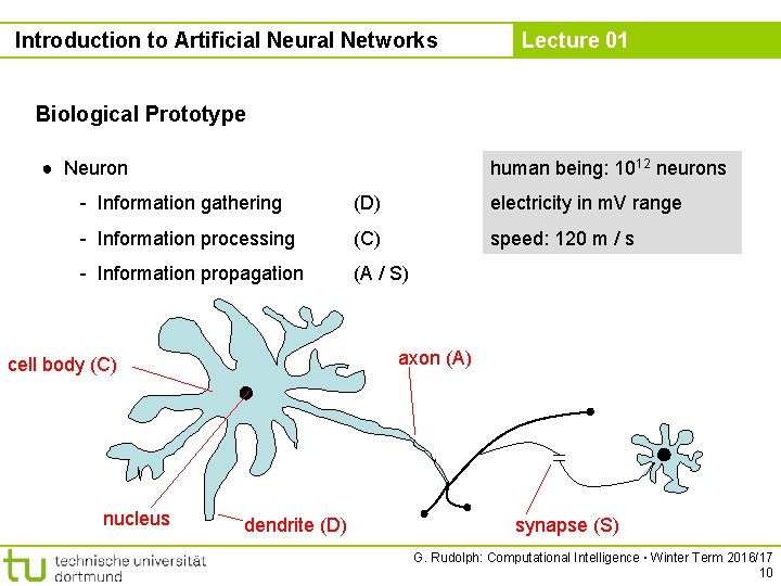
Introduction to Artificial Neural Networks Lecture 01 Biological Prototype ● Neuron human being: 1012 neurons - Information gathering (D) electricity in m. V range - Information processing (C) speed: 120 m / s - Information propagation (A / S) axon (A) cell body (C) nucleus dendrite (D) synapse (S) G. Rudolph: Computational Intelligence ▪ Winter Term 2016/17 10

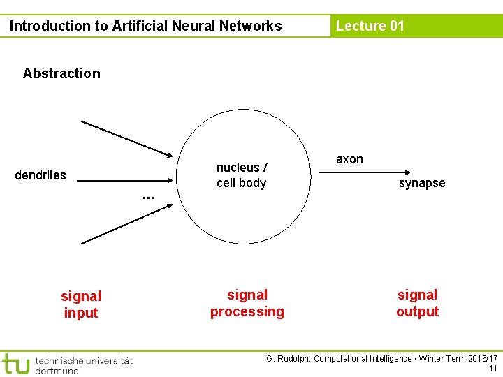
Introduction to Artificial Neural Networks Lecture 01 Abstraction dendrites … signal input nucleus / cell body signal processing axon synapse signal output G. Rudolph: Computational Intelligence ▪ Winter Term 2016/17 11

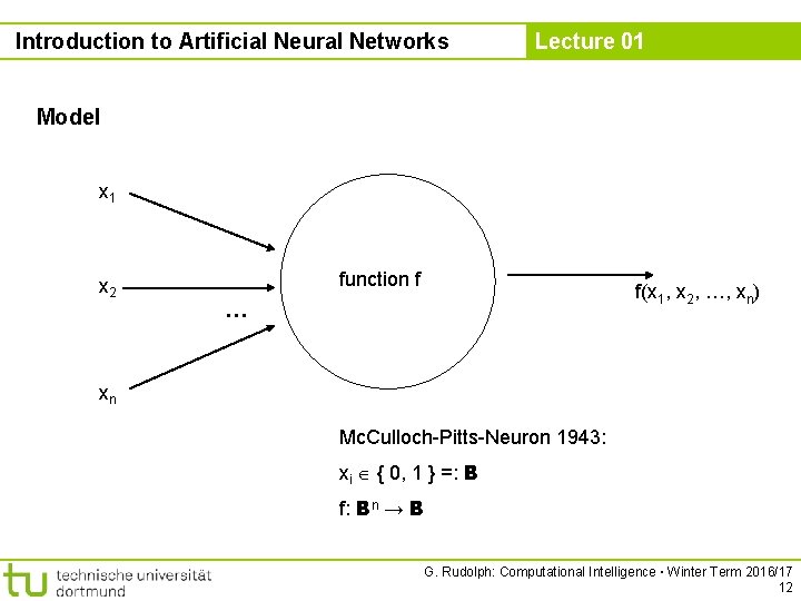
Introduction to Artificial Neural Networks Lecture 01 Model x 1 x 2 function f f(x 1, x 2, …, xn) … xn Mc. Culloch-Pitts-Neuron 1943: xi { 0, 1 } =: B f: Bn → B G. Rudolph: Computational Intelligence ▪ Winter Term 2016/17 12

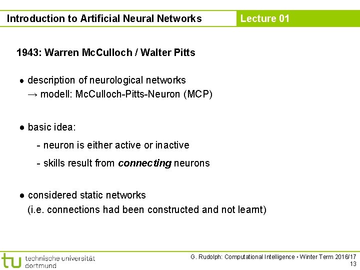
Introduction to Artificial Neural Networks Lecture 01 1943: Warren Mc. Culloch / Walter Pitts ● description of neurological networks → modell: Mc. Culloch-Pitts-Neuron (MCP) ● basic idea: - neuron is either active or inactive - skills result from connecting neurons ● considered static networks (i. e. connections had been constructed and not learnt) G. Rudolph: Computational Intelligence ▪ Winter Term 2016/17 13

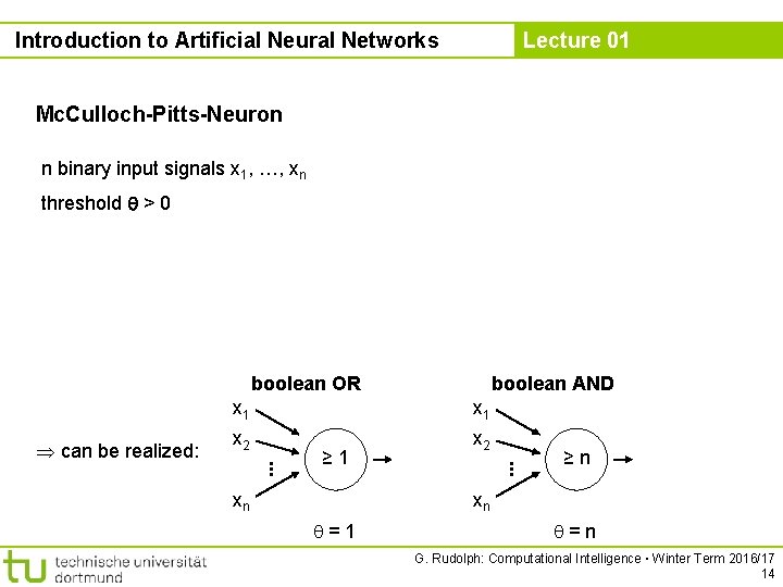
Introduction to Artificial Neural Networks Lecture 01 Mc. Culloch-Pitts-Neuron n binary input signals x 1, …, xn threshold > 0 boolean OR x 1 x 2 ≥ 1 xn . . . can be realized: boolean AND ≥n xn =1 =n G. Rudolph: Computational Intelligence ▪ Winter Term 2016/17 14

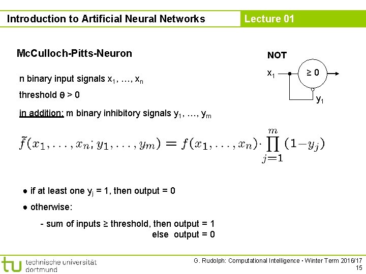
Introduction to Artificial Neural Networks Mc. Culloch-Pitts-Neuron Lecture 01 NOT x 1 n binary input signals x 1, …, xn threshold > 0 ≥ 0 y 1 in addition: m binary inhibitory signals y 1, …, ym ● if at least one yj = 1, then output = 0 ● otherwise: - sum of inputs ≥ threshold, then output = 1 else output = 0 G. Rudolph: Computational Intelligence ▪ Winter Term 2016/17 15

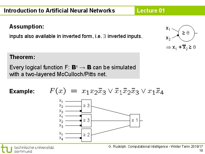
Introduction to Artificial Neural Networks Lecture 01 Assumption: x 1 inputs also available in inverted form, i. e. inverted inputs. x 2 ≥ x 1 + x 2 ≥ Theorem: Every logical function F: Bn → B can be simulated with a two-layered Mc. Culloch/Pitts net. Example: x 1 x 2 x 3 x 1 x 4 ≥ 3 ≥ 1 ≥ 2 G. Rudolph: Computational Intelligence ▪ Winter Term 2016/17 16

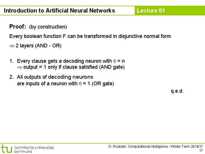
Introduction to Artificial Neural Networks Lecture 01 Proof: (by construction) Every boolean function F can be transformed in disjunctive normal form 2 layers (AND - OR) 1. Every clause gets a decoding neuron with = n output = 1 only if clause satisfied (AND gate) 2. All outputs of decoding neurons are inputs of a neuron with = 1 (OR gate) q. e. d. G. Rudolph: Computational Intelligence ▪ Winter Term 2016/17 17

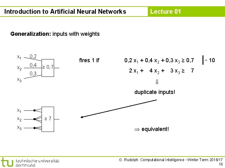
Introduction to Artificial Neural Networks Lecture 01 Generalization: inputs with weights x 1 0, 2 x 2 0, 4 fires 1 if ≥ 0, 7 0, 3 2 x 1 + 4 x 2 + 3 x 3 ≥ · 10 7 x 3 0, 2 x 1 + 0, 4 x 2 + 0, 3 x 3 ≥ 0, 7 duplicate inputs! x 1 x 2 x 3 ≥ 7 equivalent! G. Rudolph: Computational Intelligence ▪ Winter Term 2016/17 18

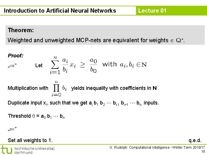
Introduction to Artificial Neural Networks Lecture 01 Theorem: Weighted and unweighted MCP-nets are equivalent for weights Q+. Proof: „ “ Let Multiplication with N yields inequality with coefficients in N Duplicate input xi, such that we get ai b 1 b 2 bi-1 bi+1 bn inputs. Threshold = a 0 b 1 bn „ “ Set all weights to 1. q. e. d. G. Rudolph: Computational Intelligence ▪ Winter Term 2016/17 19

Introduction to Artificial Neural Networks Lecture 01 Conclusion for MCP nets + feed-forward: able to compute any Boolean function + recursive: able to simulate DFA − very similar to conventional logical circuits − difficult to construct − no good learning algorithm available G. Rudolph: Computational Intelligence ▪ Winter Term 2016/17 20

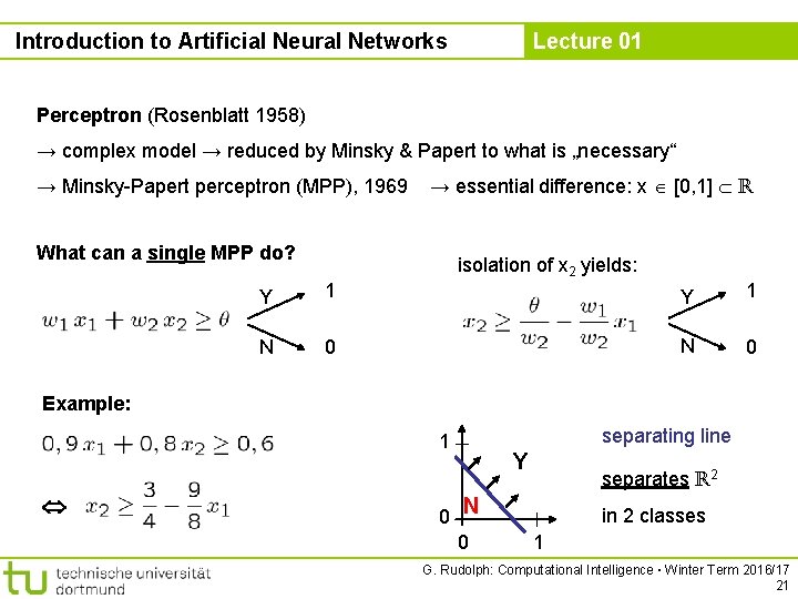
Introduction to Artificial Neural Networks Lecture 01 Perceptron (Rosenblatt 1958) → complex model → reduced by Minsky & Papert to what is „necessary“ → Minsky-Papert perceptron (MPP), 1969 → essential difference: x [0, 1] R What can a single MPP do? isolation of x 2 yields: Y 1 N 0 Example: 1 0 N 0 separating line Y separates R 2 in 2 classes 1 G. Rudolph: Computational Intelligence ▪ Winter Term 2016/17 21

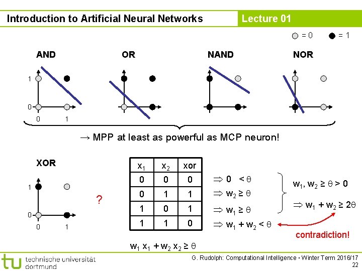
Introduction to Artificial Neural Networks Lecture 01 =0 NAND OR AND =1 NOR 1 0 0 1 → MPP at least as powerful as MCP neuron! XOR 1 ? 0 0 1 x 2 xor 0 0 1 1 1 0 0 < w 2 ≥ w 1 + w 2 < w 1 , w 2 ≥ > 0 w 1 + w 2 ≥ 2 contradiction! w 1 x 1 + w 2 x 2 ≥ G. Rudolph: Computational Intelligence ▪ Winter Term 2016/17 22

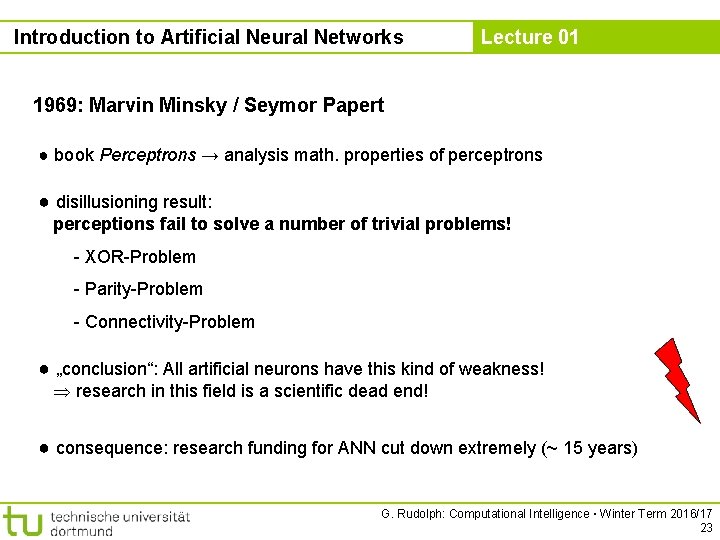
Introduction to Artificial Neural Networks Lecture 01 1969: Marvin Minsky / Seymor Papert ● book Perceptrons → analysis math. properties of perceptrons ● disillusioning result: perceptions fail to solve a number of trivial problems! - XOR-Problem - Parity-Problem - Connectivity-Problem ● „conclusion“: All artificial neurons have this kind of weakness! research in this field is a scientific dead end! ● consequence: research funding for ANN cut down extremely (~ 15 years) G. Rudolph: Computational Intelligence ▪ Winter Term 2016/17 23

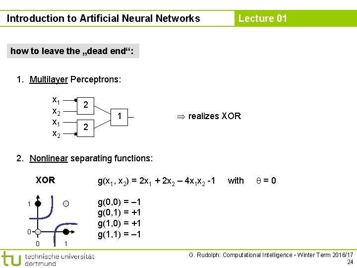
Introduction to Artificial Neural Networks Lecture 01 how to leave the „dead end“: 1. Multilayer Perceptrons: x 1 x 2 2 1 realizes XOR 2 2. Nonlinear separating functions: XOR g(x 1, x 2) = 2 x 1 + 2 x 2 – 4 x 1 x 2 -1 with =0 g(0, 0) = – 1 g(0, 1) = +1 g(1, 0) = +1 g(1, 1) = – 1 1 0 0 1 G. Rudolph: Computational Intelligence ▪ Winter Term 2016/17 24

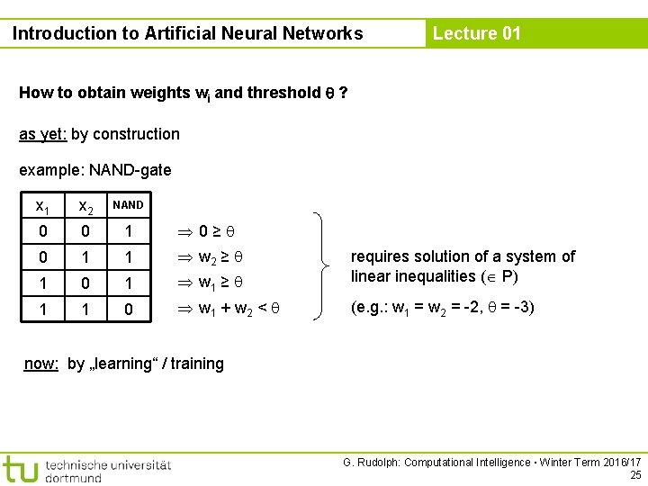
Introduction to Artificial Neural Networks Lecture 01 How to obtain weights wi and threshold ? as yet: by construction example: NAND-gate x 1 x 2 NAND 0 0 1 0≥ 0 1 1 w 2 ≥ 1 0 1 w 1 ≥ 1 1 0 w 1 + w 2 < requires solution of a system of linear inequalities ( P) (e. g. : w 1 = w 2 = -2, = -3) now: by „learning“ / training G. Rudolph: Computational Intelligence ▪ Winter Term 2016/17 25

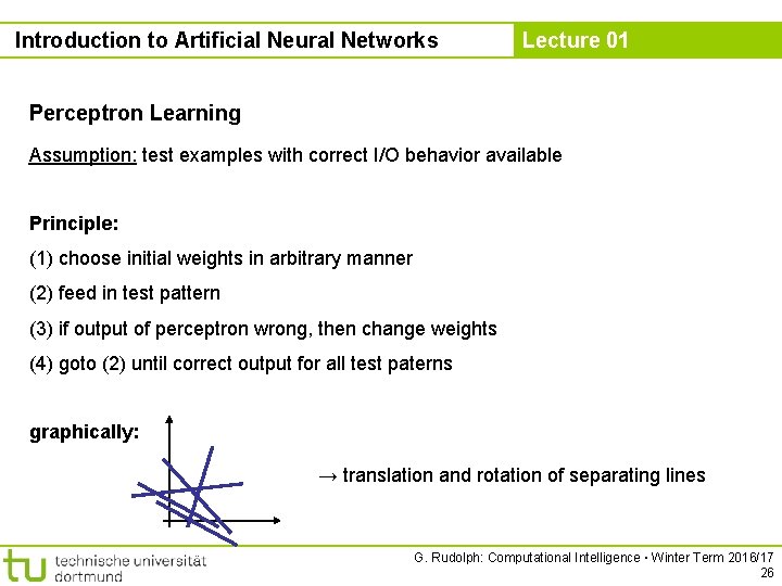
Introduction to Artificial Neural Networks Lecture 01 Perceptron Learning Assumption: test examples with correct I/O behavior available Principle: (1) choose initial weights in arbitrary manner (2) feed in test pattern (3) if output of perceptron wrong, then change weights (4) goto (2) until correct output for all test paterns graphically: → translation and rotation of separating lines G. Rudolph: Computational Intelligence ▪ Winter Term 2016/17 26

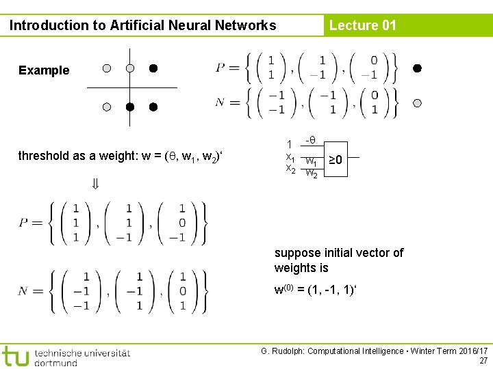
Introduction to Artificial Neural Networks Lecture 01 Example threshold as a weight: w = ( , w 1, w 2)‘ 1 - x 1 w x 2 w 1 2 ≥ 0 suppose initial vector of weights is w(0) = (1, -1, 1)‘ G. Rudolph: Computational Intelligence ▪ Winter Term 2016/17 27

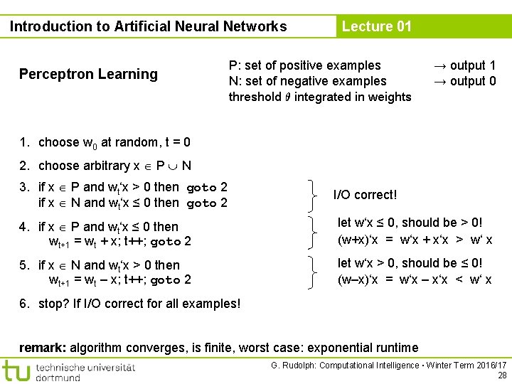
Introduction to Artificial Neural Networks Perceptron Learning Lecture 01 P: set of positive examples N: set of negative examples threshold µ integrated in weights → output 1 → output 0 1. choose w 0 at random, t = 0 2. choose arbitrary x P N 3. if x P and wt‘x > 0 then goto 2 if x N and wt‘x ≤ 0 then goto 2 I/O correct! 4. if x P and wt‘x ≤ 0 then wt+1 = wt + x; t++; goto 2 let w‘x ≤ 0, should be > 0! (w+x)‘x = w‘x + x‘x > w‘ x 5. if x N and wt‘x > 0 then wt+1 = wt – x; t++; goto 2 let w‘x > 0, should be ≤ 0! (w–x)‘x = w‘x – x‘x < w‘ x 6. stop? If I/O correct for all examples! remark: algorithm converges, is finite, worst case: exponential runtime G. Rudolph: Computational Intelligence ▪ Winter Term 2016/17 28

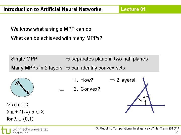
Introduction to Artificial Neural Networks Lecture 01 We know what a single MPP can do. What can be achieved with many MPPs? separates plane in two half planes Single MPP Many MPPs in 2 layers can identify convex sets 2 layers! 1. How? A B 2. Convex? a, b X: a + (1 - ) b X for (0, 1) G. Rudolph: Computational Intelligence ▪ Winter Term 2016/17 29

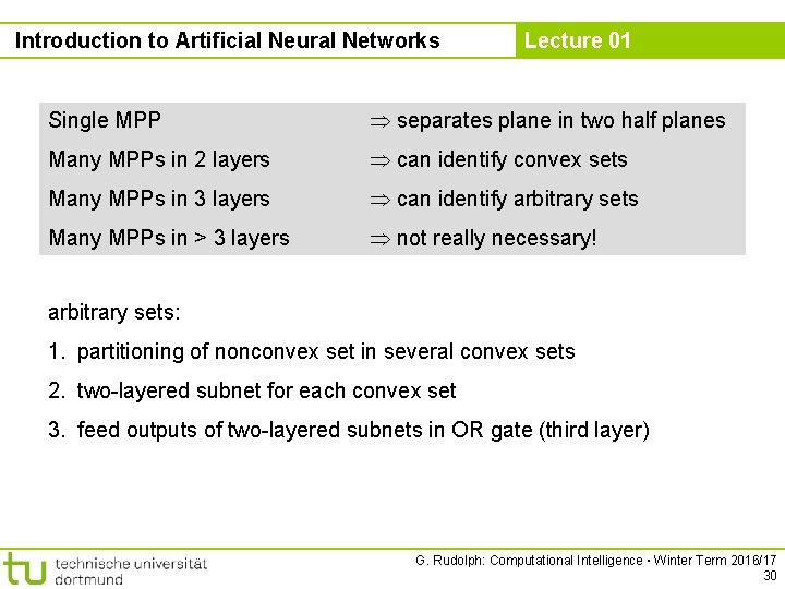
Introduction to Artificial Neural Networks Lecture 01 Single MPP separates plane in two half planes Many MPPs in 2 layers can identify convex sets Many MPPs in 3 layers can identify arbitrary sets Many MPPs in > 3 layers not really necessary! arbitrary sets: 1. partitioning of nonconvex set in several convex sets 2. two-layered subnet for each convex set 3. feed outputs of two-layered subnets in OR gate (third layer) G. Rudolph: Computational Intelligence ▪ Winter Term 2016/17 30