Computational Intelligence Winter Term 201617 Prof Dr Gnter

Computational Intelligence Winter Term 2016/17 Prof. Dr. Günter Rudolph Lehrstuhl für Algorithm Engineering (LS 11) Fakultät für Informatik TU Dortmund

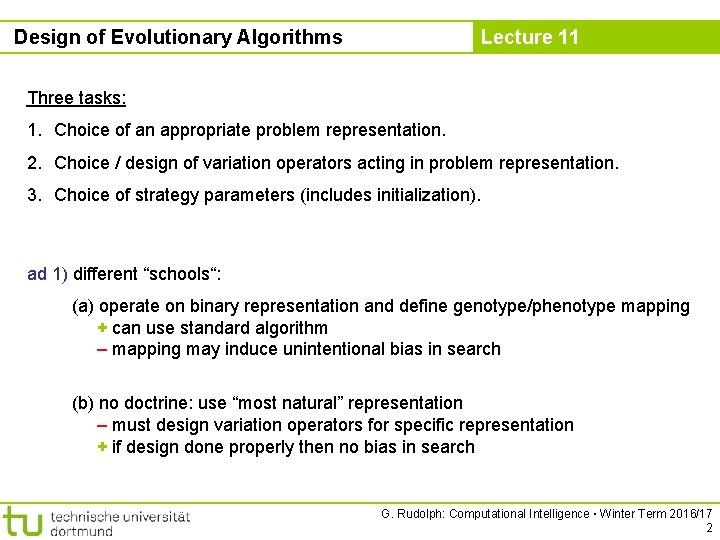
Design of Evolutionary Algorithms Lecture 11 Three tasks: 1. Choice of an appropriate problem representation. 2. Choice / design of variation operators acting in problem representation. 3. Choice of strategy parameters (includes initialization). ad 1) different “schools“: (a) operate on binary representation and define genotype/phenotype mapping + can use standard algorithm – mapping may induce unintentional bias in search (b) no doctrine: use “most natural” representation – must design variation operators for specific representation + if design done properly then no bias in search G. Rudolph: Computational Intelligence ▪ Winter Term 2016/17 2

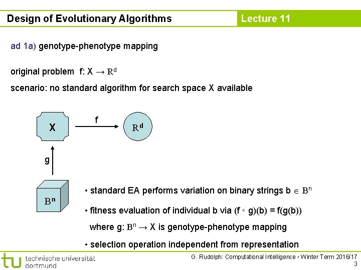
Design of Evolutionary Algorithms Lecture 11 ad 1 a) genotype-phenotype mapping original problem f: X → Rd scenario: no standard algorithm for search space X available X f Rd g • standard EA performs variation on binary strings b Bn Bn • fitness evaluation of individual b via (f ◦ g)(b) = f(g(b)) where g: Bn → X is genotype-phenotype mapping • selection operation independent from representation G. Rudolph: Computational Intelligence ▪ Winter Term 2016/17 3

Design of Evolutionary Algorithms Lecture 11 Genotype-Phenotype-Mapping Bn → [L, R] R ● Standard encoding for b Bn → Problem: hamming cliffs 000 001 010 011 100 101 110 111 genotype 0 1 2 3 4 5 6 7 phenotype 1 Bit 2 Bit 1 Bit 3 Bit 1 Bit Hamming cliff 2 Bit 1 Bit L = 0, R = 7 n=3 G. Rudolph: Computational Intelligence ▪ Winter Term 2016/17 4

Design of Evolutionary Algorithms Lecture 11 Genotype-Phenotype-Mapping Bn → [L, R] R ● Gray encoding for b Bn Let a Bn ai, standard encoded. Then bi = if i = 1 ai-1 ai, if i > 1 = XOR 000 001 010 111 100 genotype 0 1 2 3 4 5 6 7 phenotype OK, no hamming cliffs any longer … small changes in phenotype „lead to“ small changes in genotype since we consider evolution in terms of Darwin (not Lamarck): small changes in genotype lead to small changes in phenotype! but: 1 -Bit-change: 000 → 100 G. Rudolph: Computational Intelligence ▪ Winter Term 2016/17 5

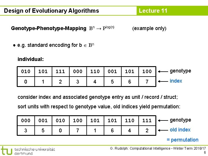
Design of Evolutionary Algorithms Lecture 11 Genotype-Phenotype-Mapping Bn → Plog(n) (example only) ● e. g. standard encoding for b Bn individual: 010 101 111 000 110 001 100 0 1 2 3 4 5 6 7 genotype index consider index and associated genotype entry as unit / record / struct; sort units with respect to genotype value, old indices yield permutation: 000 001 010 101 101 110 111 genotype 3 5 0 7 1 6 4 2 old index = permutation G. Rudolph: Computational Intelligence ▪ Winter Term 2016/17 6

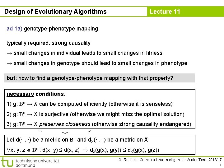
Design of Evolutionary Algorithms Lecture 11 ad 1 a) genotype-phenotype mapping typically required: strong causality → small changes in individual leads to small changes in fitness → small changes in genotype should lead to small changes in phenotype but: how to find a genotype-phenotype mapping with that property? necessary conditions: 1) g: Bn → X can be computed efficiently (otherwise it is senseless) 2) g: Bn → X is surjective (otherwise we might miss the optimal solution) 3) g: Bn → X preserves closeness (otherwise strong causality endangered) Let d(· , ·) be a metric on Bn and d. X(· , ·) be a metric on X. x, y, z Bn : d(x, y) ≤ d(x, z) d. X(g(x), g(y)) ≤ d. X(g(x), g(z)) G. Rudolph: Computational Intelligence ▪ Winter Term 2016/17 7

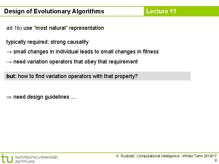
Design of Evolutionary Algorithms Lecture 11 ad 1 b) use “most natural“ representation typically required: strong causality → small changes in individual leads to small changes in fitness → need variation operators that obey that requirement but: how to find variation operators with that property? need design guidelines. . . G. Rudolph: Computational Intelligence ▪ Winter Term 2016/17 8

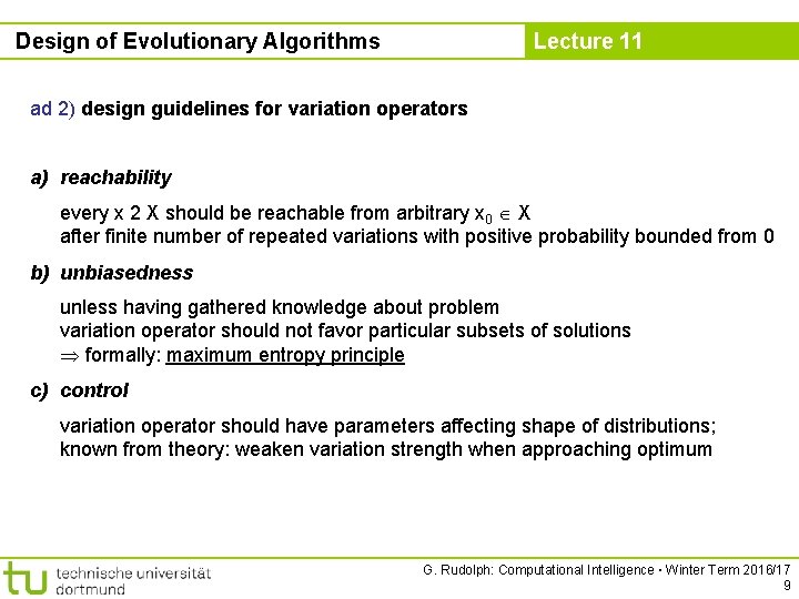
Design of Evolutionary Algorithms Lecture 11 ad 2) design guidelines for variation operators a) reachability every x 2 X should be reachable from arbitrary x 0 X after finite number of repeated variations with positive probability bounded from 0 b) unbiasedness unless having gathered knowledge about problem variation operator should not favor particular subsets of solutions formally: maximum entropy principle c) control variation operator should have parameters affecting shape of distributions; known from theory: weaken variation strength when approaching optimum G. Rudolph: Computational Intelligence ▪ Winter Term 2016/17 9

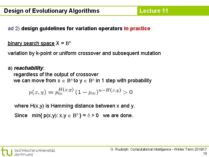
Design of Evolutionary Algorithms Lecture 11 ad 2) design guidelines for variation operators in practice binary search space X = Bn variation by k-point or uniform crossover and subsequent mutation a) reachability: regardless of the output of crossover we can move from x Bn to y Bn in 1 step with probability where H(x, y) is Hamming distance between x and y. Since min{ p(x, y): x, y Bn } = > 0 we are done. G. Rudolph: Computational Intelligence ▪ Winter Term 2016/17 10

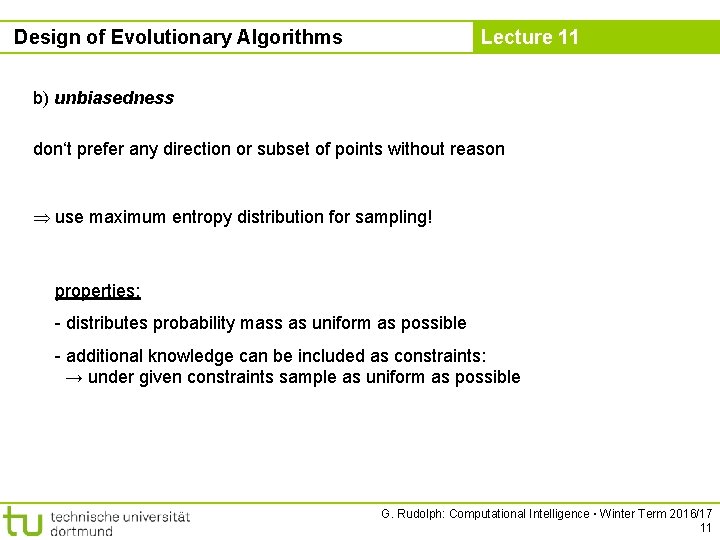
Design of Evolutionary Algorithms Lecture 11 b) unbiasedness don‘t prefer any direction or subset of points without reason use maximum entropy distribution for sampling! properties: - distributes probability mass as uniform as possible - additional knowledge can be included as constraints: → under given constraints sample as uniform as possible G. Rudolph: Computational Intelligence ▪ Winter Term 2016/17 11

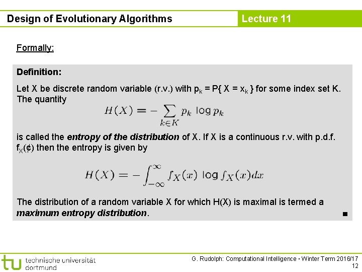
Design of Evolutionary Algorithms Lecture 11 Formally: Definition: Let X be discrete random variable (r. v. ) with pk = P{ X = xk } for some index set K. The quantity is called the entropy of the distribution of X. If X is a continuous r. v. with p. d. f. f. X(¢) then the entropy is given by The distribution of a random variable X for which H(X) is maximal is termed a maximum entropy distribution. ■ G. Rudolph: Computational Intelligence ▪ Winter Term 2016/17 12

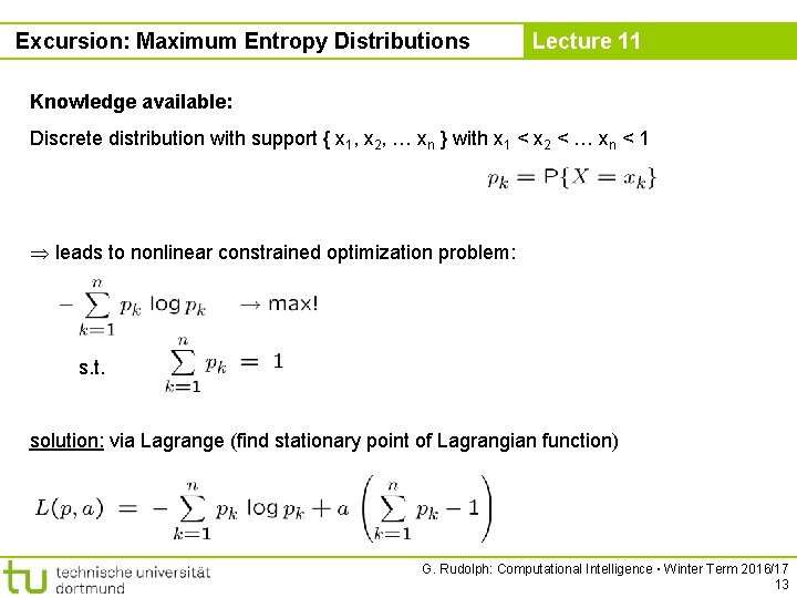
Excursion: Maximum Entropy Distributions Lecture 11 Knowledge available: Discrete distribution with support { x 1, x 2, … xn } with x 1 < x 2 < … xn < 1 leads to nonlinear constrained optimization problem: s. t. solution: via Lagrange (find stationary point of Lagrangian function) G. Rudolph: Computational Intelligence ▪ Winter Term 2016/17 13

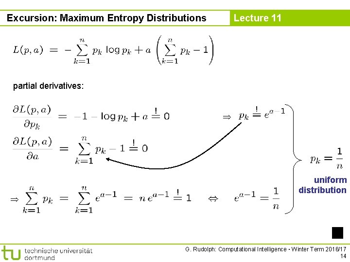
Excursion: Maximum Entropy Distributions Lecture 11 partial derivatives: uniform distribution G. Rudolph: Computational Intelligence ▪ Winter Term 2016/17 14

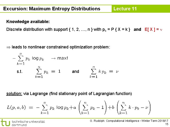
Excursion: Maximum Entropy Distributions Lecture 11 Knowledge available: Discrete distribution with support { 1, 2, …, n } with pk = P { X = k } and E[ X ] = leads to nonlinear constrained optimization problem: s. t. and solution: via Lagrange (find stationary point of Lagrangian function) G. Rudolph: Computational Intelligence ▪ Winter Term 2016/17 15

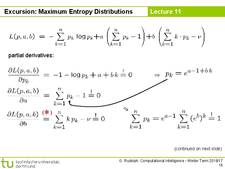
Excursion: Maximum Entropy Distributions Lecture 11 partial derivatives: *) ( (continued on next slide) G. Rudolph: Computational Intelligence ▪ Winter Term 2016/17 16

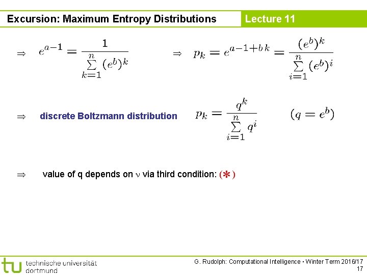
Excursion: Maximum Entropy Distributions Lecture 11 discrete Boltzmann distribution *) value of q depends on via third condition: ( G. Rudolph: Computational Intelligence ▪ Winter Term 2016/17 17

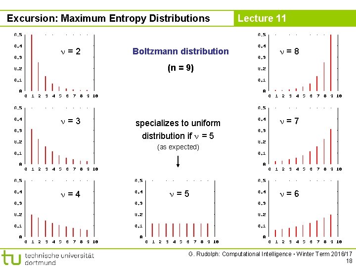
Excursion: Maximum Entropy Distributions =2 Boltzmann distribution Lecture 11 =8 (n = 9) =3 specializes to uniform distribution if = 5 =7 (as expected) =4 =5 =6 G. Rudolph: Computational Intelligence ▪ Winter Term 2016/17 18

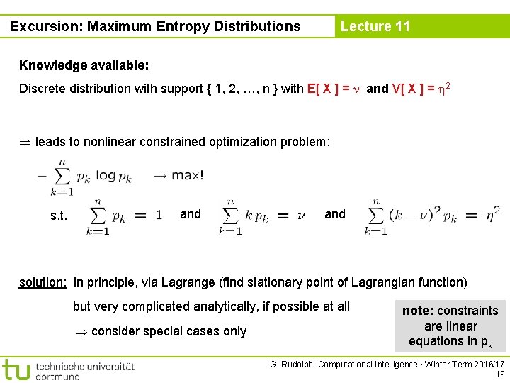
Excursion: Maximum Entropy Distributions Lecture 11 Knowledge available: Discrete distribution with support { 1, 2, …, n } with E[ X ] = and V[ X ] = 2 leads to nonlinear constrained optimization problem: s. t. and solution: in principle, via Lagrange (find stationary point of Lagrangian function) but very complicated analytically, if possible at all consider special cases only note: constraints are linear equations in pk G. Rudolph: Computational Intelligence ▪ Winter Term 2016/17 19

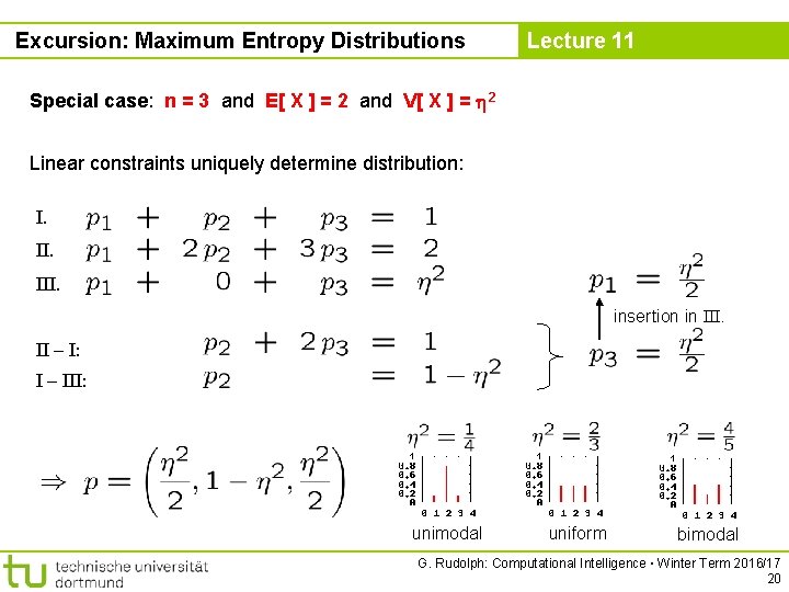
Excursion: Maximum Entropy Distributions Lecture 11 Special case: n = 3 and E[ X ] = 2 and V[ X ] = 2 Linear constraints uniquely determine distribution: I. III. insertion in III. II – I: I – III: unimodal uniform bimodal G. Rudolph: Computational Intelligence ▪ Winter Term 2016/17 20

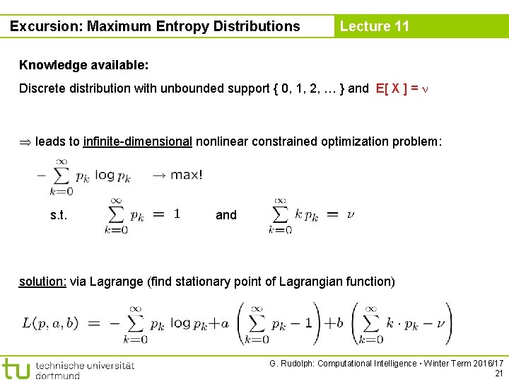
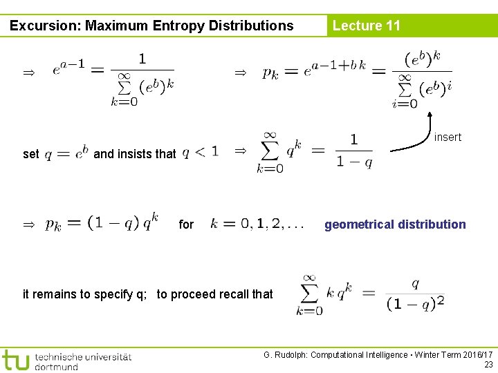
Excursion: Maximum Entropy Distributions Lecture 11 Knowledge available: Discrete distribution with unbounded support { 0, 1, 2, … } and E[ X ] = leads to infinite-dimensional nonlinear constrained optimization problem: s. t. and solution: via Lagrange (find stationary point of Lagrangian function) G. Rudolph: Computational Intelligence ▪ Winter Term 2016/17 21

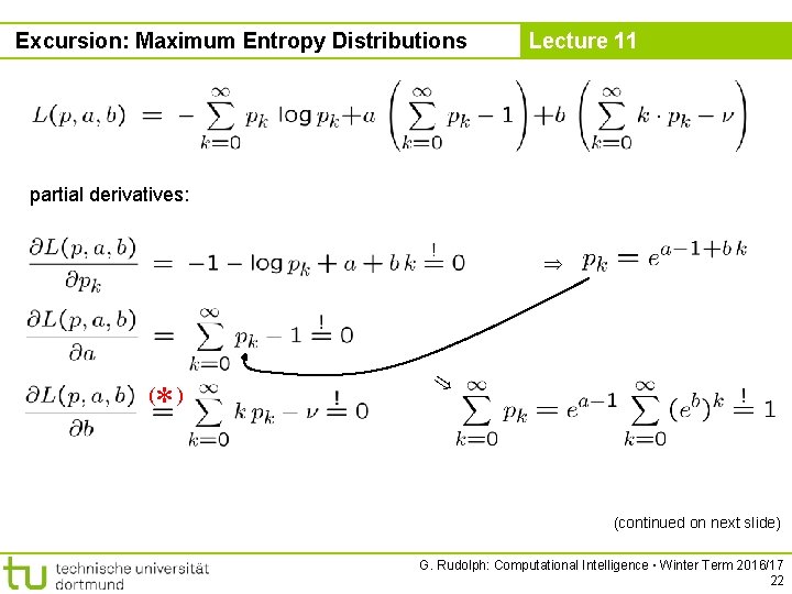
Excursion: Maximum Entropy Distributions Lecture 11 partial derivatives: *) ( (continued on next slide) G. Rudolph: Computational Intelligence ▪ Winter Term 2016/17 22

Excursion: Maximum Entropy Distributions set Lecture 11 insert and insists that for geometrical distribution it remains to specify q; to proceed recall that G. Rudolph: Computational Intelligence ▪ Winter Term 2016/17 23

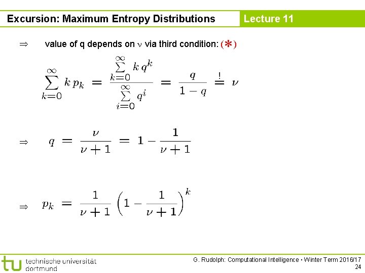
Excursion: Maximum Entropy Distributions Lecture 11 *) value of q depends on via third condition: ( G. Rudolph: Computational Intelligence ▪ Winter Term 2016/17 24

Excursion: Maximum Entropy Distributions =1 Lecture 11 =7 geometrical distribution with E[ x ] = =2 =6 pk only shown for k = 0, 1, …, 8 =3 =4 =5 G. Rudolph: Computational Intelligence ▪ Winter Term 2016/17 25

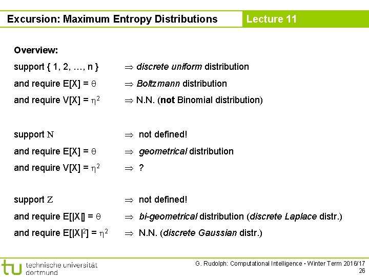
Excursion: Maximum Entropy Distributions Lecture 11 Overview: support { 1, 2, …, n } discrete uniform distribution and require E[X] = Boltzmann distribution and require V[X] = 2 N. N. (not Binomial distribution) support N not defined! and require E[X] = geometrical distribution and require V[X] = 2 ? support Z not defined! and require E[|X|] = bi-geometrical distribution (discrete Laplace distr. ) and require E[|X|2] = 2 N. N. (discrete Gaussian distr. ) G. Rudolph: Computational Intelligence ▪ Winter Term 2016/17 26

Excursion: Maximum Entropy Distributions Lecture 11 support [a, b] R uniform distribution support R+ with E[X] = Exponential distribution support R with E[X] = , V[X] = 2 normal / Gaussian distribution N( , 2) support Rn with E[X] = and Cov[X] = C multinormal distribution N( , C) expectation vector Rn covariance matrix Rn, n positive definite: x ≠ 0 : x‘Cx > 0 G. Rudolph: Computational Intelligence ▪ Winter Term 2016/17 27

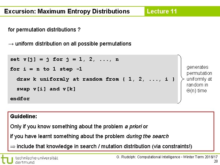
Excursion: Maximum Entropy Distributions Lecture 11 for permutation distributions ? → uniform distribution on all possible permutations set v[j] = j for j = 1, 2, . . . , n for i = n to 1 step -1 draw k uniformly at random from { 1, 2, . . . , i } swap v[i] and v[k] generates permutation uniformly at random in (n) time endfor Guideline: Only if you know something about the problem a priori or if you have learnt something about the problem during the search include that knowledge in search / mutation distribution (via constraints!) G. Rudolph: Computational Intelligence ▪ Winter Term 2016/17 28

Design of Evolutionary Algorithms Lecture 11 ad 2) design guidelines for variation operators in practice integer search space X = Zn a) reachability b) unbiasedness c) control - every recombination results in some z Zn - mutation of z may then lead to any z* Zn with positive probability in one step ad a) support of mutation should be Zn ad b) need maximum entropy distribution over support Zn ad c) control variability by parameter → formulate as constraint of maximum entropy distribution G. Rudolph: Computational Intelligence ▪ Winter Term 2016/17 29

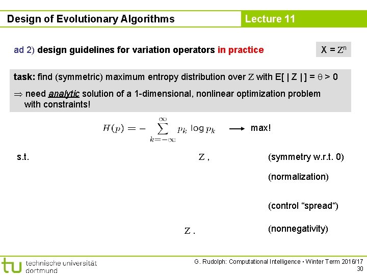
Design of Evolutionary Algorithms Lecture 11 X = Zn ad 2) design guidelines for variation operators in practice task: find (symmetric) maximum entropy distribution over Z with E[ | Z | ] = > 0 need analytic solution of a 1 -dimensional, nonlinear optimization problem with constraints! max! Z, s. t. (symmetry w. r. t. 0) (normalization) (control “spread“) Z. (nonnegativity) G. Rudolph: Computational Intelligence ▪ Winter Term 2016/17 30

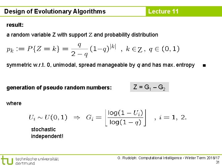
Design of Evolutionary Algorithms Lecture 11 result: a random variable Z with support Z and probability distribution Z symmetric w. r. t. 0, unimodal, spread manageable by q and has max. entropy generation of pseudo random numbers: ■ Z = G 1 – G 2 where stochastic independent! G. Rudolph: Computational Intelligence ▪ Winter Term 2016/17 31

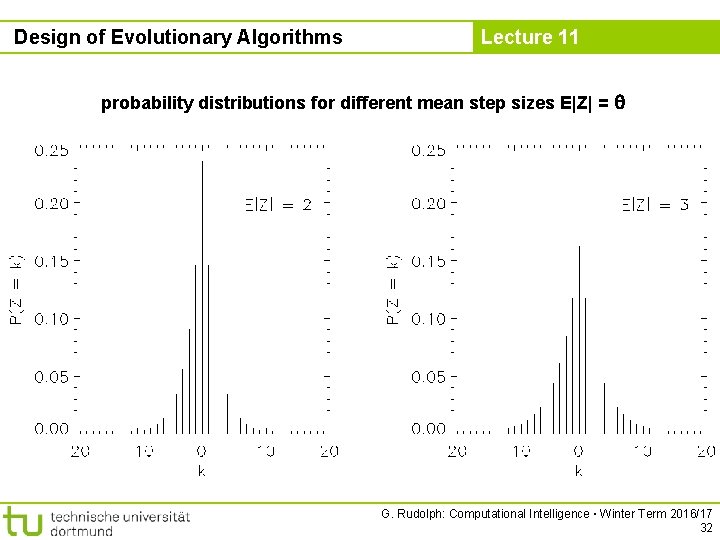
Design of Evolutionary Algorithms Lecture 11 probability distributions for different mean step sizes E|Z| = G. Rudolph: Computational Intelligence ▪ Winter Term 2016/17 32

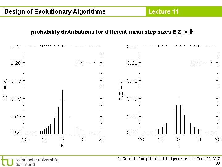
Design of Evolutionary Algorithms Lecture 11 probability distributions for different mean step sizes E|Z| = G. Rudolph: Computational Intelligence ▪ Winter Term 2016/17 33

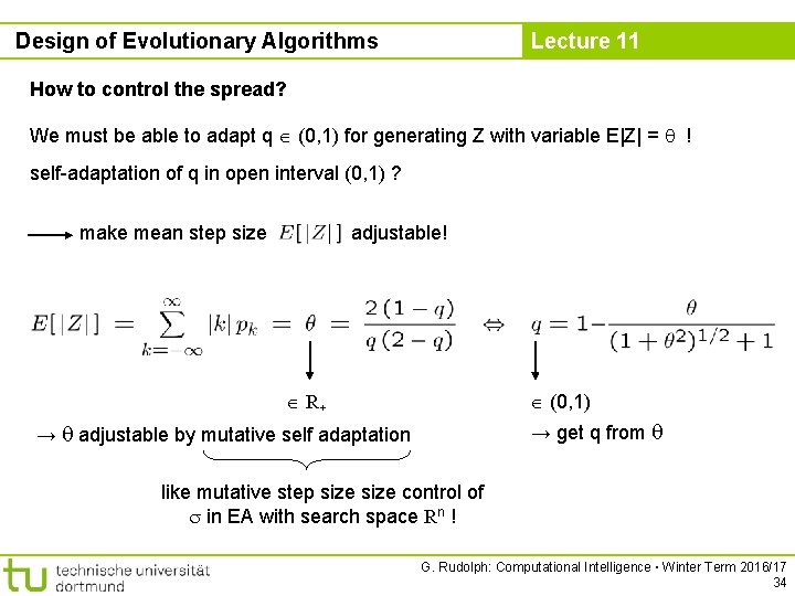
Design of Evolutionary Algorithms Lecture 11 How to control the spread? We must be able to adapt q (0, 1) for generating Z with variable E|Z| = ! self-adaptation of q in open interval (0, 1) ? make mean step size adjustable! R+ (0, 1) → get q from → adjustable by mutative self adaptation like mutative step size control of in EA with search space Rn ! G. Rudolph: Computational Intelligence ▪ Winter Term 2016/17 34

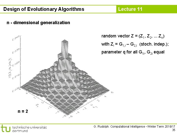
Design of Evolutionary Algorithms Lecture 11 n - dimensional generalization random vector Z = (Z 1, Z 2, . . . Zn) with Zi = G 1, i – G 2, i (stoch. indep. ); parameter q for all G 1 i, G 2 i equal n=2 G. Rudolph: Computational Intelligence ▪ Winter Term 2016/17 35

Design of Evolutionary Algorithms Lecture 11 n - dimensional generalization n-dimensional distribution is symmetric w. r. t. 1 norm! all random vectors with same step length have same probability! G. Rudolph: Computational Intelligence ▪ Winter Term 2016/17 36

Design of Evolutionary Algorithms Lecture 11 How to control E[ || Z ||1 ] ? by def. linearity of E[·] identical distributions for Zi = self-adaptation calculate from G. Rudolph: Computational Intelligence ▪ Winter Term 2016/17 37

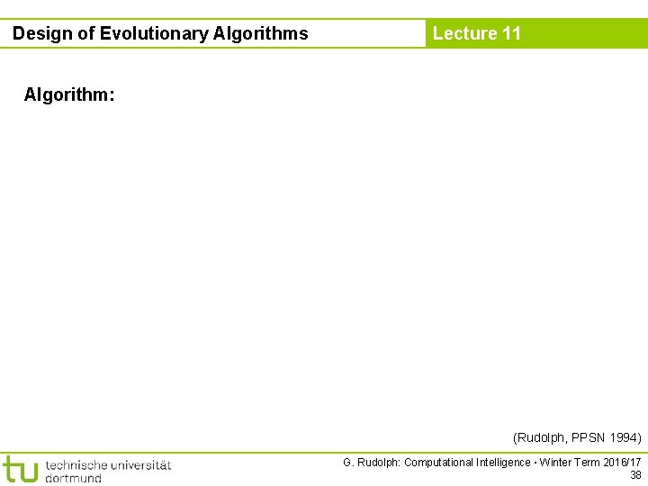
Design of Evolutionary Algorithms Lecture 11 Algorithm: (Rudolph, PPSN 1994) G. Rudolph: Computational Intelligence ▪ Winter Term 2016/17 38

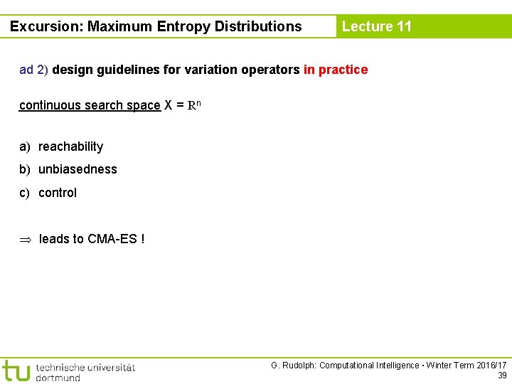
Excursion: Maximum Entropy Distributions Lecture 11 ad 2) design guidelines for variation operators in practice continuous search space X = Rn a) reachability b) unbiasedness c) control leads to CMA-ES ! G. Rudolph: Computational Intelligence ▪ Winter Term 2016/17 39