Computational Intelligence Methods and Applications Lecture 3 Histograms

Computational Intelligence: Methods and Applications Lecture 3 Histograms and probabilities. Włodzisław Duch Dept. of Informatics, UMK Google: W Duch

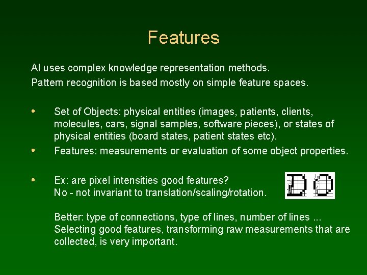
Features AI uses complex knowledge representation methods. Pattern recognition is based mostly on simple feature spaces. • • • Set of Objects: physical entities (images, patients, clients, molecules, cars, signal samples, software pieces), or states of physical entities (board states, patient states etc). Features: measurements or evaluation of some object properties. Ex: are pixel intensities good features? No - not invariant to translation/scaling/rotation. Better: type of connections, type of lines, number of lines. . . Selecting good features, transforming raw measurements that are collected, is very important.

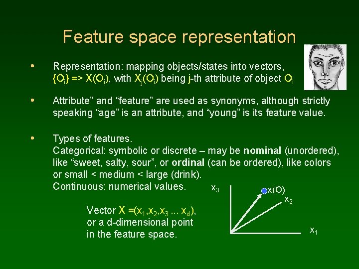
Feature space representation • Representation: mapping objects/states into vectors, {Oi} => X(Oi), with Xj(Oi) being j-th attribute of object Oi • Attribute” and “feature” are used as synonyms, although strictly speaking “age” is an attribute, and “young” is its feature value. • Types of features. Categorical: symbolic or discrete – may be nominal (unordered), like “sweet, salty, sour”, or ordinal (can be ordered), like colors or small < medium < large (drink). Continuous: numerical values. x 3 x(O) Vector X =(x 1, x 2, x 3. . . xd), or a d-dimensional point in the feature space. x 2 x 1

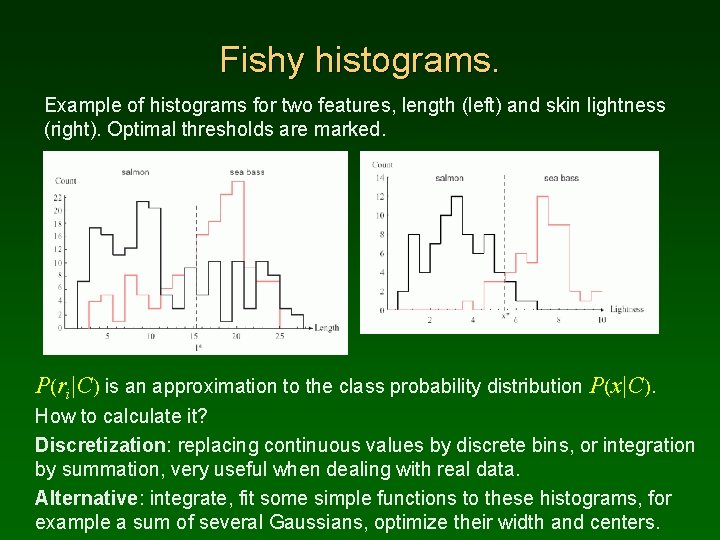
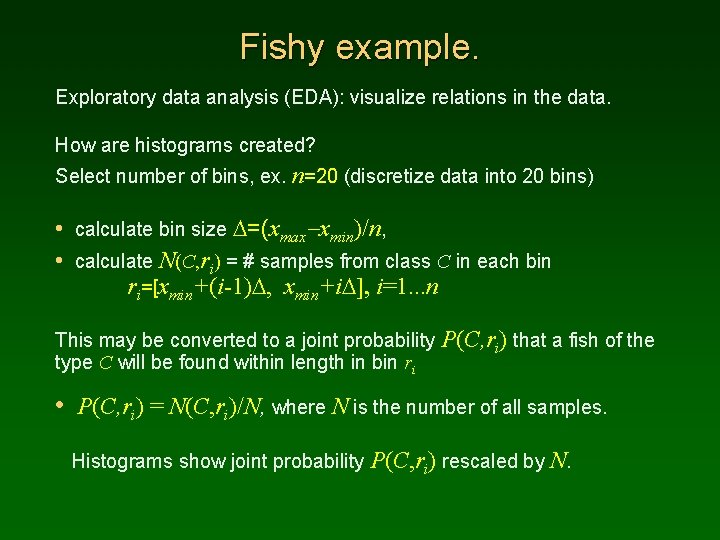
Fishy example. Chapter 1. 2, Pattern Classification (2 nd ed) by R. O. Duda, P. E. Hart and D. G. Stork, John Wiley & Sons, 2000 Singapore Fisheries automates the process of sorting salmon and sea bass fish, coming on a conveyor belt. Optical sensor and processing software evaluate a number of features: length, lightness, width, #fins Step 1: look at the histograms. • Select number of bins, ex. n=20 (discretize data) • calculate bin size D=(xmax- xmin)/n, • calculate N(C, ri) = # samples in class C {salmon, bass} in each bin ri = [xmin+(i-1)D, xmin+i. D], i=1. . . n • normalize P(C, ri)=N(C, ri)/N, where N is the number of all samples. This gives joint probability P(C, ri) = P(ri|C)P(C)

Fishy histograms. Example of histograms for two features, length (left) and skin lightness (right). Optimal thresholds are marked. P(ri|C) is an approximation to the class probability distribution P(x|C). How to calculate it? Discretization: replacing continuous values by discrete bins, or integration by summation, very useful when dealing with real data. Alternative: integrate, fit some simple functions to these histograms, for example a sum of several Gaussians, optimize their width and centers.

Fishy example. Exploratory data analysis (EDA): visualize relations in the data. How are histograms created? Select number of bins, ex. n=20 (discretize data into 20 bins) • calculate bin size D=(xmax-xmin)/n, • calculate N(C, ri) = # samples from class C in each bin ri=[xmin+(i-1)D, xmin+i. D], i=1. . . n This may be converted to a joint probability P(C, ri) that a fish of the type C will be found within length in bin ri • P(C, ri) = N(C, ri)/N, where N is the number of all samples. Histograms show joint probability P(C, ri) rescaled by N.

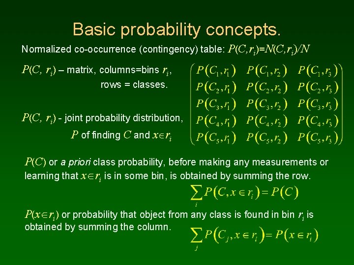
Basic probability concepts. Normalized co-occurrence (contingency) table: P(C, ri)=N(C, ri)/N P(C, ri) – matrix, columns=bins ri, rows = classes. P(C, ri) - joint probability distribution, P of finding C and x ri P(C) or a priori class probability, before making any measurements or learning that x ri is in some bin, is obtained by summing the row. P(x ri) or probability that object from any class is found in bin ri is obtained by summing the column.

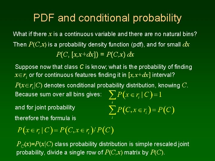
PDF and conditional probability What if there x is a continuous variable and there are no natural bins? Then P(C, x) is a probability density function (pdf), and for small dx P(C, [x, x+dx]) = P(C, x) dx Suppose now that class C is know; what is the probability of finding x ri or for continuous features finding it in [x, x+dx] interval? P(x ri|C) denotes conditional probability distribution, knowing C. Because sum over all bins gives: and for joint probability therefore the formula is PC(x)=P(x|C) class probability distribution is simple rescaled joint probability, divide a single row of P(C, x) matrix by P(C).

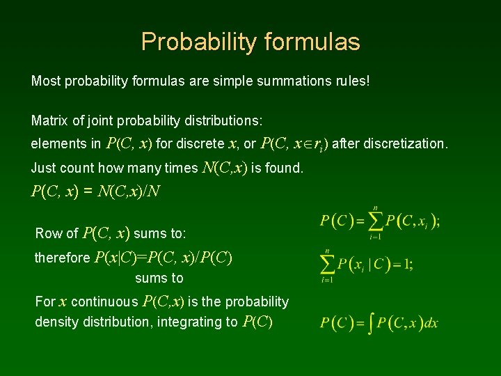
Probability formulas Most probability formulas are simple summations rules! Matrix of joint probability distributions: elements in P(C, x) for discrete x, or P(C, x ri) after discretization. Just count how many times N(C, x) is found. P(C, x) = N(C, x)/N Row of P(C, x) sums to: therefore P(x|C)=P(C, x)/P(C) sums to For x continuous P(C, x) is the probability density distribution, integrating to P(C)

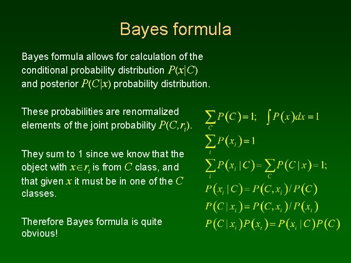
Bayes formula allows for calculation of the conditional probability distribution P(x|C) and posterior P(C|x) probability distribution. These probabilities are renormalized elements of the joint probability P(C, ri). They sum to 1 since we know that the object with x ri is from C class, and that given x it must be in one of the C classes. Therefore Bayes formula is quite obvious!

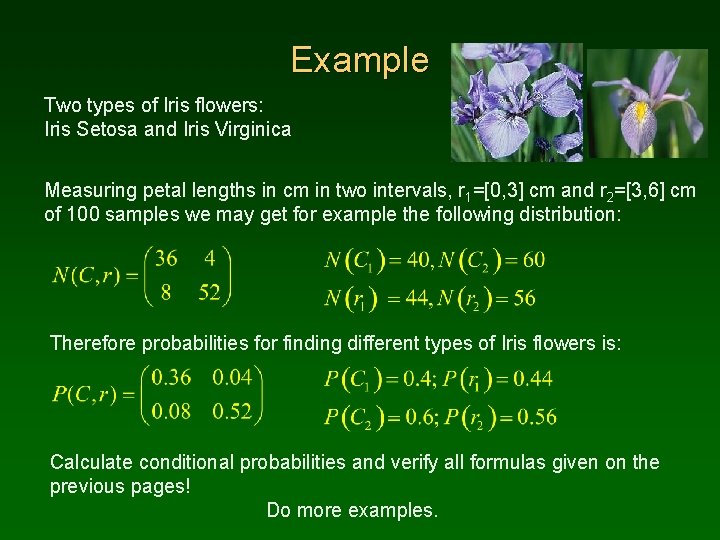
Example Two types of Iris flowers: Iris Setosa and Iris Virginica Measuring petal lengths in cm in two intervals, r 1=[0, 3] cm and r 2=[3, 6] cm of 100 samples we may get for example the following distribution: Therefore probabilities for finding different types of Iris flowers is: Calculate conditional probabilities and verify all formulas given on the previous pages! Do more examples.

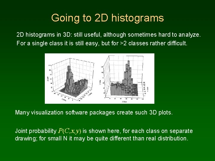
Going to 2 D histograms in 3 D: still useful, although sometimes hard to analyze. For a single class it is still easy, but for >2 classes rather difficult. Many visualization software packages create such 3 D plots. Joint probability P(C, x, y) is shown here, for each class on separate drawing; for small N it may be quite different than real distribution.

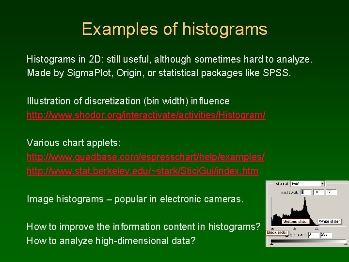
Examples of histograms Histograms in 2 D: still useful, although sometimes hard to analyze. Made by Sigma. Plot, Origin, or statistical packages like SPSS. Illustration of discretization (bin width) influence http: //www. shodor. org/interactivate/activities/Histogram/ Various chart applets: http: //www. quadbase. com/espresschart/help/examples/ http: //www. stat. berkeley. edu/~stark/Stici. Gui/index. htm Image histograms – popular in electronic cameras. How to improve the information content in histograms? How to analyze high-dimensional data?

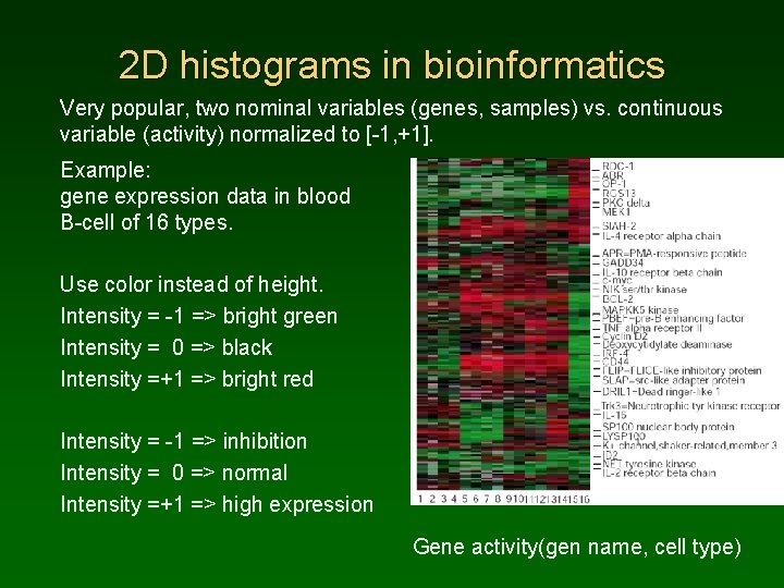
2 D histograms in bioinformatics Very popular, two nominal variables (genes, samples) vs. continuous variable (activity) normalized to [-1, +1]. Example: gene expression data in blood B-cell of 16 types. Use color instead of height. Intensity = -1 => bright green Intensity = 0 => black Intensity =+1 => bright red Intensity = -1 => inhibition Intensity = 0 => normal Intensity =+1 => high expression Gene activity(gen name, cell type)