Computational Intelligence Methods and Applications Lecture 27 Expectation

Computational Intelligence: Methods and Applications Lecture 27 Expectation Maximization algorithm, density modeling Włodzisław Duch Dept. of Informatics, UMK Google: W Duch

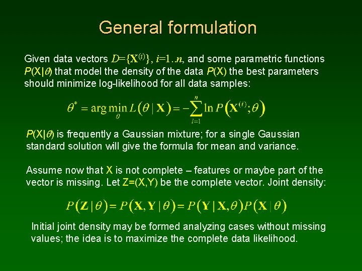
General formulation Given data vectors D={X(i)}, i=1. . n, and some parametric functions P(X|q) that model the density of the data P(X) the best parameters should minimize log-likelihood for all data samples: P(X|q) is frequently a Gaussian mixture; for a single Gaussian standard solution will give the formula for mean and variance. Assume now that X is not complete – features or maybe part of the vector is missing. Let Z=(X, Y) be the complete vector. Joint density: Initial joint density may be formed analyzing cases without missing values; the idea is to maximize the complete data likelihood.

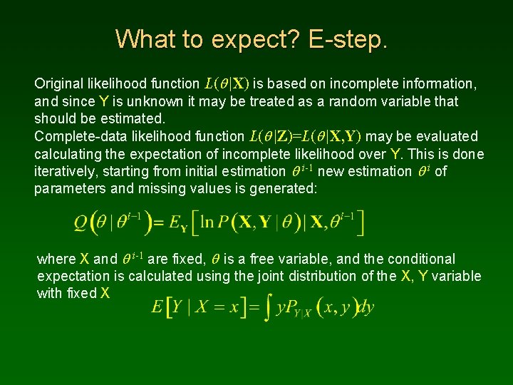
What to expect? E-step. Original likelihood function L(q |X) is based on incomplete information, and since Y is unknown it may be treated as a random variable that should be estimated. Complete-data likelihood function L(q |Z)=L(q |X, Y) may be evaluated calculating the expectation of incomplete likelihood over Y. This is done iteratively, starting from initial estimation q i-1 new estimation q i of parameters and missing values is generated: where X and q i-1 are fixed, q is a free variable, and the conditional expectation is calculated using the joint distribution of the X, Y variable with fixed X

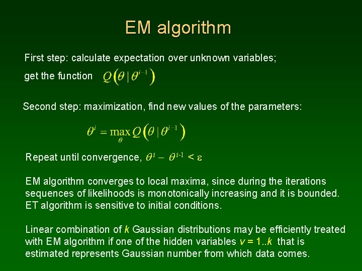
EM algorithm First step: calculate expectation over unknown variables; get the function Second step: maximization, find new values of the parameters: Repeat until convergence, q i - q i-1 < e EM algorithm converges to local maxima, since during the iterations sequences of likelihoods is monotonically increasing and it is bounded. ET algorithm is sensitive to initial conditions. Linear combination of k Gaussian distributions may be efficiently treated with EM algorithm if one of the hidden variables v = 1. . k that is estimated represents Gaussian number from which data comes.

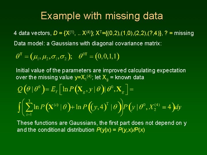
Example with missing data 4 data vectors, D = {X(1), . . X(4)}; XT={(0, 2), (1, 0), (2, 2), (? , 4)}, ? = missing Data model: a Gaussians with diagonal covariance matrix: Initial value of the parameters are improved calculating expectation over the missing value y=X 1(4); let Xg = known data These functions are Gaussians, the first part does not depend on y and the conditional distribution P(y|x) = P(y, x)/P(x)

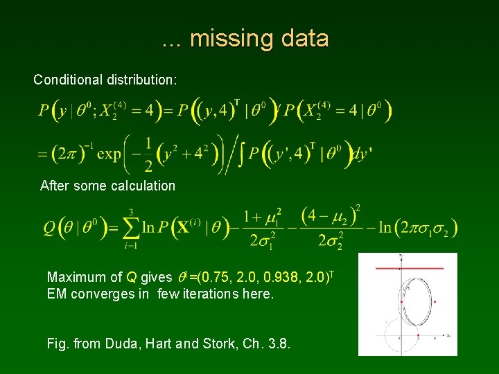
. . . missing data Conditional distribution: After some calculation Maximum of Q gives q 1=(0. 75, 2. 0, 0. 938, 2. 0)T EM converges in few iterations here. Fig. from Duda, Hart and Stork, Ch. 3. 8.

Some applications • Reconstruction of missing values. • Reconstruction of images, many medical applications. • Reconstruction of signals in the presence of noise. • Unsupervised learning – no information about classes is needed, more than clustering, natural taxonomy. • Modeling of data, estimation of hidden parameters in mixtures. • Training of probabilistic models, such as HMM (Hidden Markov models), useful in speech recognition, bioinformatics. . . Associative memory, finding the whole pattern (image) after seeing a fragment – although I have never seen it yet done with EM. . . Book: Geoffrey J. Mc. Lachlan, Thriyambakam Krishnan, The EM Algorithm and Extensions, Wiley 1996

EM demos Few demonstration of the EM algorithm for Gaussian mixtures may be found in the network. http: //www-cse. ucsd. edu/users/ibayrakt/java/em/ http: //www. neurosci. aist. go. jp/~akaho/Mixture. EM. html EM is also a basis for “multiple imputation” approach to missing data. Each missing datum is replaced by m>1 simulated values and m versions of the complete data analyzed by standard methods; results are combined to produce inferential statements that incorporate missing -data uncertainty. Schafer, JL (1997) Analysis of Incomplete Multivariate Data, Chapman & Hall. Some demo software is available: http: //www. stat. psu. edu/~jls/misoftwa. html Demonstration of EM in WEKA for clustering data.