Computational Intelligence Methods and Applications Lecture 5 EDA

Computational Intelligence: Methods and Applications Lecture 5 EDA and linear transformations. Włodzisław Duch Dept. of Informatics, UMK Google: W Duch

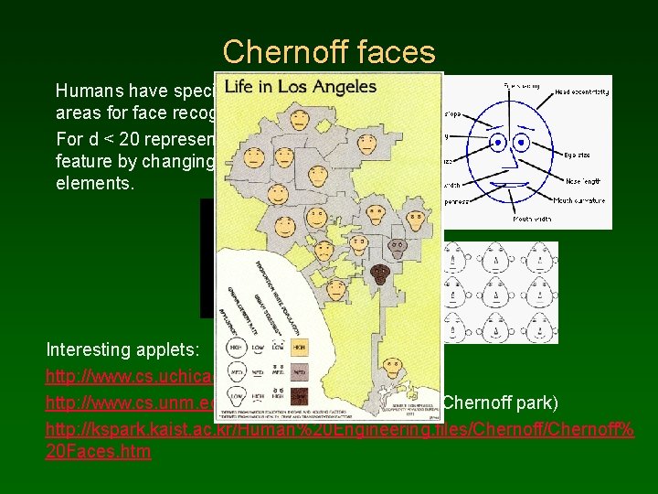
Chernoff faces Humans have specialized brain areas for face recognition. For d < 20 represent each feature by changing some face elements. Interesting applets: http: //www. cs. uchicago. edu/~wiseman/chernoff/ http: //www. cs. unm. edu/~dlchao/flake/chernoff/ (Chernoff park) http: //kspark. kaist. ac. kr/Human%20 Engineering. files/Chernoff% 20 Faces. htm

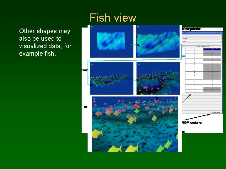
Fish view Other shapes may also be used to visualized data, for example fish.

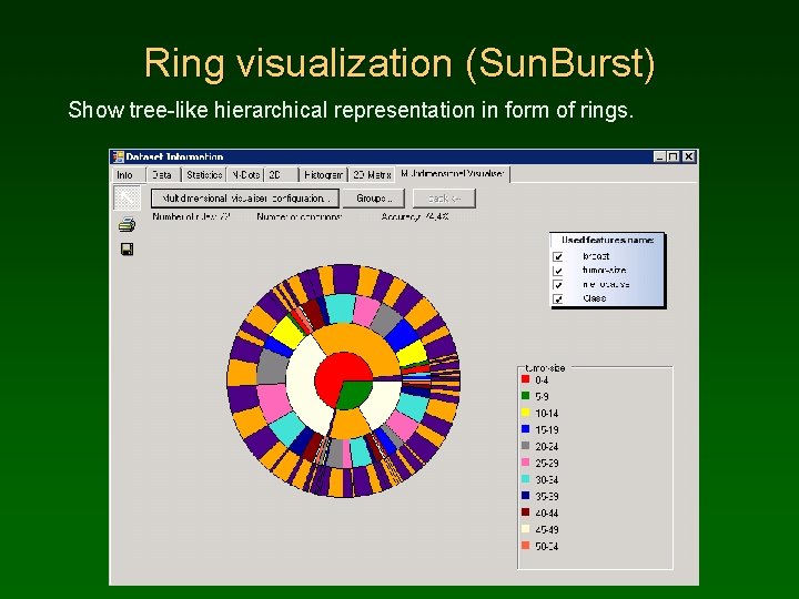
Ring visualization (Sun. Burst) Show tree-like hierarchical representation in form of rings.

Other EDA techniques NIST Engineering Statistics Handbook has a chapter on exploratory data analysis (EDA). http: //www. itl. nist. gov/div 898/handbook/index. htm Unfortunately many visualization programs are written for X-Windows only, are in Fortran, or S or R languages. Sonification: data converted to sounds! Example: sound of EEG data. Java Voice Think about potential applications! More: http: //sonification. de/ http: //en. wikipedia. org/wiki/Sonification

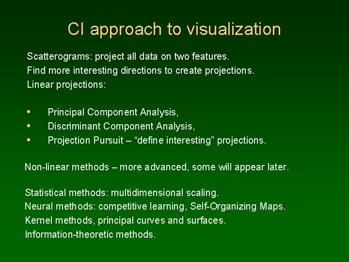
CI approach to visualization Scatterograms: project all data on two features. Find more interesting directions to create projections. Linear projections: • • • Principal Component Analysis, Discriminant Component Analysis, Projection Pursuit – “define interesting” projections. Non-linear methods – more advanced, some will appear later. Statistical methods: multidimensional scaling. Neural methods: competitive learning, Self-Organizing Maps. Kernel methods, principal curves and surfaces. Information-theoretic methods.

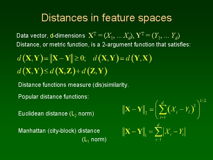
Distances in feature spaces Data vector, d-dimensions XT = (X 1, . . . Xd), YT = (Y 1, . . . Yd) Distance, or metric function, is a 2 -argument function that satisfies: Distance functions measure (dis)similarity. Popular distance functions: Euclidean distance (L 2 norm) Manhattan (city-block) distance (L 1 norm)

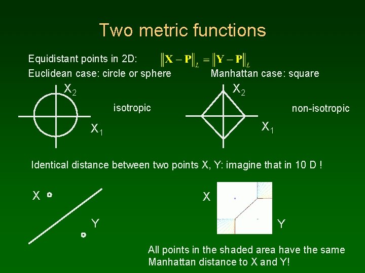
Two metric functions Equidistant points in 2 D: Euclidean case: circle or sphere Manhattan case: square X 2 isotropic non-isotropic X 1 Identical distance between two points X, Y: imagine that in 10 D ! X X Y Y All points in the shaded area have the same Manhattan distance to X and Y!

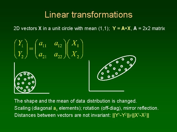
Linear transformations 2 D vectors X in a unit circle with mean (1, 1); Y = A*X, A = 2 x 2 matrix The shape and the mean of data distribution is changed. Scaling (diagonal aii elements); rotation (off-diag), mirror reflection. Distances between vectors are not invariant: ||Y 1 -Y 2||≠||X 1 -X 2||

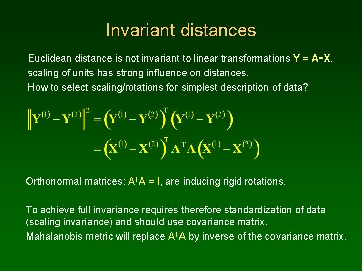
Invariant distances Euclidean distance is not invariant to linear transformations Y = A*X, scaling of units has strong influence on distances. How to select scaling/rotations for simplest description of data? Orthonormal matrices: ATA = I, are inducing rigid rotations. To achieve full invariance requires therefore standardization of data (scaling invariance) and should use covariance matrix. Mahalanobis metric will replace ATA by inverse of the covariance matrix.

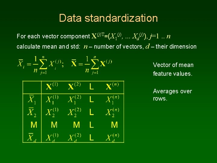
Data standardization For each vector component X(j)T=(X 1(j), . . . Xd(j)), j=1. . n calculate mean and std: n – number of vectors, d – their dimension Vector of mean feature values. Averages over rows.

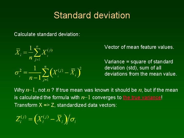
Standard deviation Calculate standard deviation: Vector of mean feature values. Variance = square of standard deviation (std), sum of all deviations from the mean value. Why n-1, not n ? If true mean was known it should be n, but if the mean is calculated the formula with n-1 converges to the true variance! Transform X => Z, standardized data vectors:

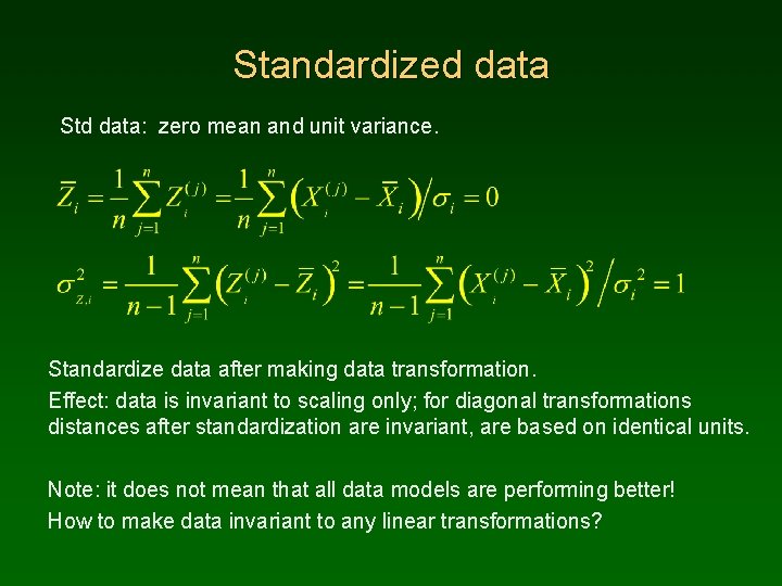
Standardized data Std data: zero mean and unit variance. Standardize data after making data transformation. Effect: data is invariant to scaling only; for diagonal transformations distances after standardization are invariant, are based on identical units. Note: it does not mean that all data models are performing better! How to make data invariant to any linear transformations?

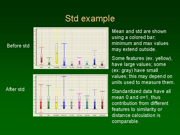
Std example Before std Mean and std are shown using a colored bar; minimum and max values may extend outside. Some features (ex. yellow), have large values; some (ex: gray) have small values; this may depend on units used to measure them. After std Standardized data have all mean 0 and s=1, thus contribution from different features to similarity or distance calculation is comparable.