CMSC 341 Asymptotic Analysis Complexity How many resources

CMSC 341 Asymptotic Analysis

Complexity How many resources will it take to solve a problem of a given size? – time – space Expressed as a function of problem size (beyond some minimum size) – how do requirements grow as size grows? Problem size – number of elements to be handled – size of thing to be operated on 2

Mileage Example Problem: John drives his car, how much gas does he use? 3

The Goal of Asymptotic Analysis How to analyze the running time (aka computational complexity) of an algorithm in a theoretical model. Using a theoretical model allows us to ignore the effects of – Which computer are we using? – How good is our compiler at optimization We define the running time of an algorithm with input size n as T ( n ) and examine the rate of growth of T( n ) as n grows larger and larger. 4

Growth Functions Constant T(n) = c ex: getting array element at known location trying on a shirt calling a friend for fashion advice Linear T(n) = cn [+ possible lower order terms] ex: finding particular element in array (sequential search) trying on all your shirts calling all your n friends for fashion advice 5

Growth Functions (cont) Quadratic T(n) = cn 2 [ + possible lower order terms] ex: sorting all the elements in an array (using bubble sort) trying all your shirts (n) with all your ties (n) having conference calls with each pair of n friends Polynomial T(n) = cnk [ + possible lower order terms] ex: looking for maximum substrings in array trying on all combinations of k separates types of apparels (n of each) having conferences calls with each k-tuple of n friends 6

Growth Functions (cont) Exponential T(n) = cn [+ possible lower order terms] ex: constructing all possible orders of array elements Logarithmic T(n) = logn [ + possible lower order terms] ex: finding a particular array element (binary search) trying on all Garanimal combinations getting fashion advice from n friends using phone tree 7

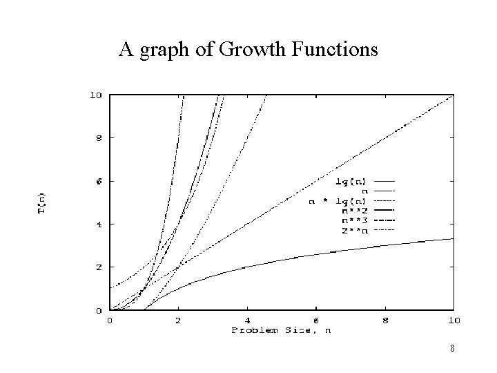
A graph of Growth Functions 8

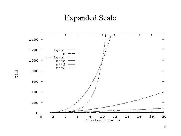
Expanded Scale 9

Asymptotic Analysis What happens as problem size grows really, really large? (in the limit) – constants don’t matter – lower order terms don’t matter 10

Analysis Cases What particular input (of given size) gives worst/best/average complexity? Mileage example: how much gas does it take to go 20 miles? – Worst case: all uphill – Best case: all downhill, just coast – Average case: “average terrain” 11

Cases Example Consider sequential search on an unsorted array of length n, what is time complexity? Best case: Worst case: Average case: 12

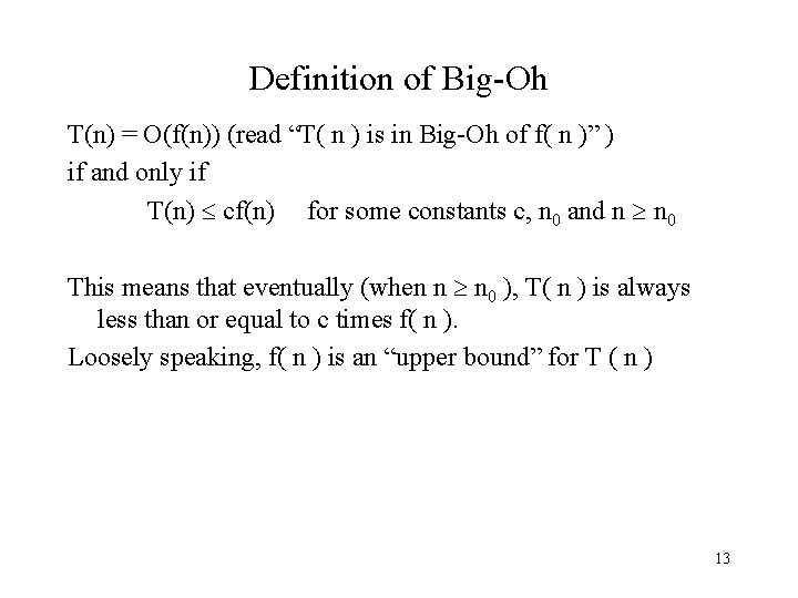
Definition of Big-Oh T(n) = O(f(n)) (read “T( n ) is in Big-Oh of f( n )” ) if and only if T(n) cf(n) for some constants c, n 0 and n n 0 This means that eventually (when n n 0 ), T( n ) is always less than or equal to c times f( n ). Loosely speaking, f( n ) is an “upper bound” for T ( n ) 13

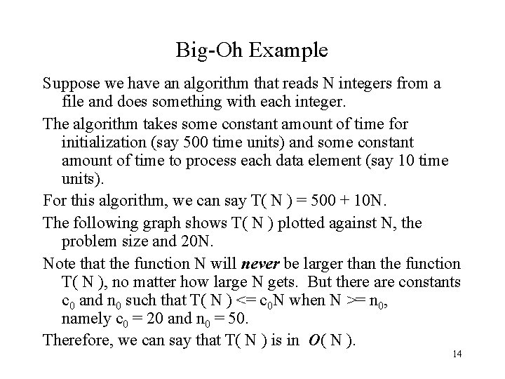
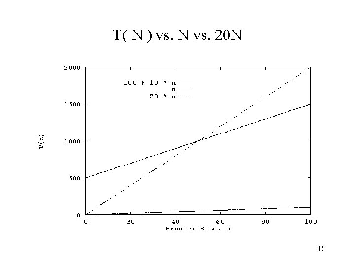
Big-Oh Example Suppose we have an algorithm that reads N integers from a file and does something with each integer. The algorithm takes some constant amount of time for initialization (say 500 time units) and some constant amount of time to process each data element (say 10 time units). For this algorithm, we can say T( N ) = 500 + 10 N. The following graph shows T( N ) plotted against N, the problem size and 20 N. Note that the function N will never be larger than the function T( N ), no matter how large N gets. But there are constants c 0 and n 0 such that T( N ) <= c 0 N when N >= n 0, namely c 0 = 20 and n 0 = 50. Therefore, we can say that T( N ) is in O( N ). 14

T( N ) vs. N vs. 20 N 15

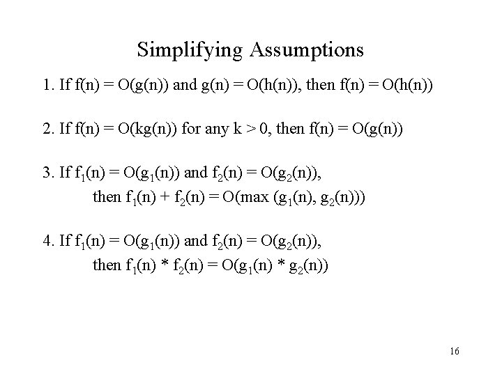
Simplifying Assumptions 1. If f(n) = O(g(n)) and g(n) = O(h(n)), then f(n) = O(h(n)) 2. If f(n) = O(kg(n)) for any k > 0, then f(n) = O(g(n)) 3. If f 1(n) = O(g 1(n)) and f 2(n) = O(g 2(n)), then f 1(n) + f 2(n) = O(max (g 1(n), g 2(n))) 4. If f 1(n) = O(g 1(n)) and f 2(n) = O(g 2(n)), then f 1(n) * f 2(n) = O(g 1(n) * g 2(n)) 16

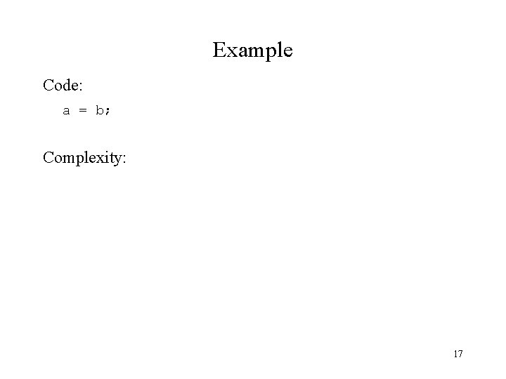
Example Code: a = b; Complexity: 17

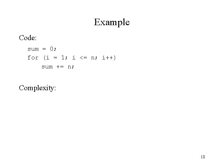
Example Code: sum = 0; for (i = 1; i <= n; i++) sum += n; Complexity: 18

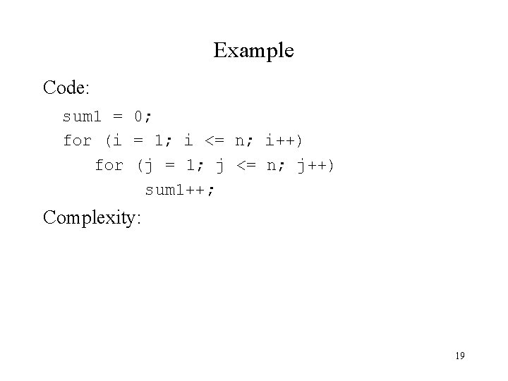
Example Code: sum 1 = 0; for (i = 1; i <= n; i++) for (j = 1; j <= n; j++) sum 1++; Complexity: 19

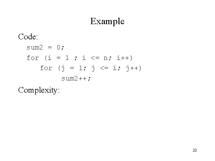
Example Code: sum 2 = 0; for (i = 1 ; i <= n; i++) for (j = 1; j <= i; j++) sum 2++; Complexity: 20

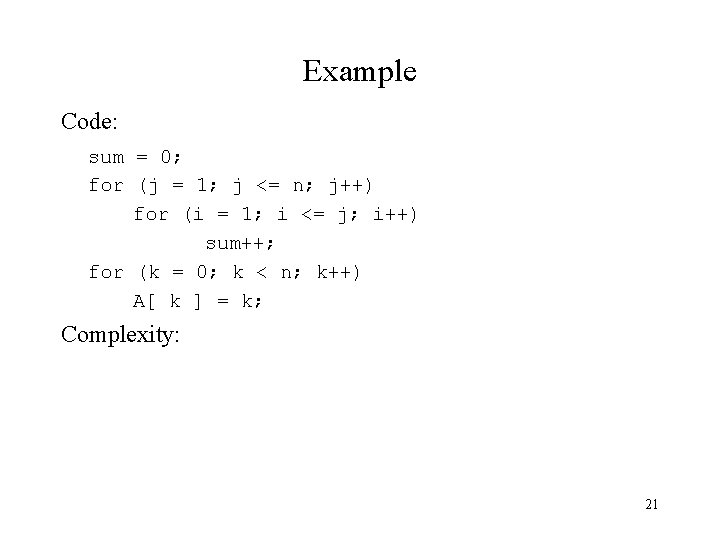
Example Code: sum = 0; for (j = 1; j <= n; j++) for (i = 1; i <= j; i++) sum++; for (k = 0; k < n; k++) A[ k ] = k; Complexity: 21

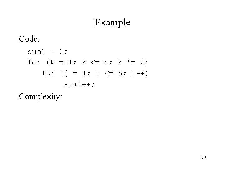
Example Code: sum 1 = 0; for (k = 1; k <= n; k *= 2) for (j = 1; j <= n; j++) sum 1++; Complexity: 22

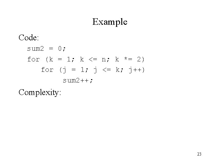
Example Code: sum 2 = 0; for (k = 1; k <= n; k *= 2) for (j = 1; j <= k; j++) sum 2++; Complexity: 23

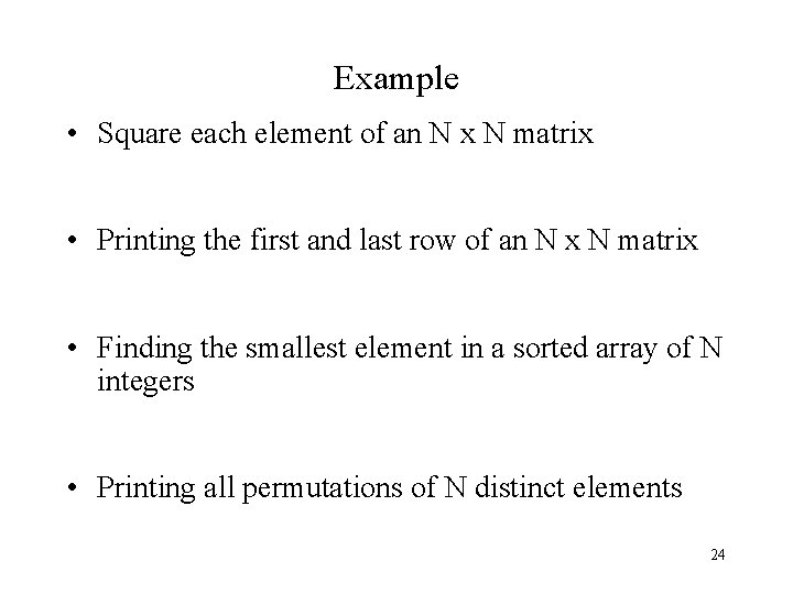
Example • Square each element of an N x N matrix • Printing the first and last row of an N x N matrix • Finding the smallest element in a sorted array of N integers • Printing all permutations of N distinct elements 24

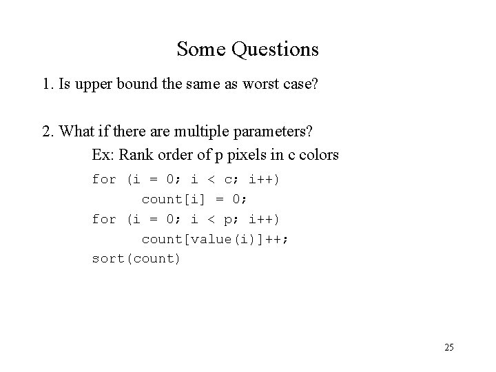
Some Questions 1. Is upper bound the same as worst case? 2. What if there are multiple parameters? Ex: Rank order of p pixels in c colors for (i = 0; i < c; i++) count[i] = 0; for (i = 0; i < p; i++) count[value(i)]++; sort(count) 25

Space Complexity Does it matter? What determines space complexity? How can you reduce it? What tradeoffs are involved? 26

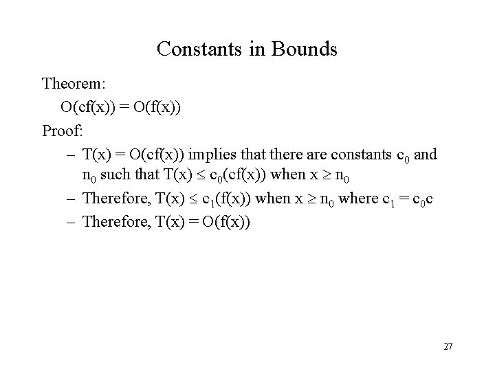
Constants in Bounds Theorem: O(cf(x)) = O(f(x)) Proof: – T(x) = O(cf(x)) implies that there are constants c 0 and n 0 such that T(x) c 0(cf(x)) when x n 0 – Therefore, T(x) c 1(f(x)) when x n 0 where c 1 = c 0 c – Therefore, T(x) = O(f(x)) 27

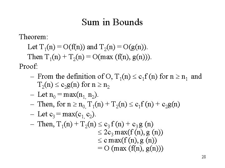
Sum in Bounds Theorem: Let T 1(n) = O(f(n)) and T 2(n) = O(g(n)). Then T 1(n) + T 2(n) = O(max (f(n), g(n))). Proof: – From the definition of O, T 1(n) c 1 f (n) for n n 1 and T 2(n) c 2 g(n) for n n 2 – Let n 0 = max(n 1, n 2). – Then, for n n 0, T 1(n) + T 2(n) c 1 f (n) + c 2 g(n) – Let c 3 = max(c 1, c 2). – Then, T 1(n) + T 2(n) c 3 f (n) + c 3 g (n) 2 c 3 max(f (n), g (n)) c max(f (n), g (n)) = O (max (f(n), g(n))) 28

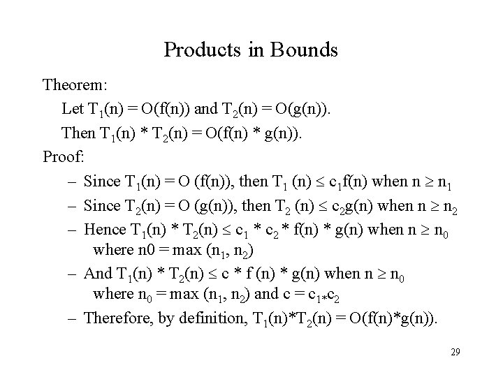
Products in Bounds Theorem: Let T 1(n) = O(f(n)) and T 2(n) = O(g(n)). Then T 1(n) * T 2(n) = O(f(n) * g(n)). Proof: – Since T 1(n) = O (f(n)), then T 1 (n) c 1 f(n) when n n 1 – Since T 2(n) = O (g(n)), then T 2 (n) c 2 g(n) when n n 2 – Hence T 1(n) * T 2(n) c 1 * c 2 * f(n) * g(n) when n n 0 where n 0 = max (n 1, n 2) – And T 1(n) * T 2(n) c * f (n) * g(n) when n n 0 where n 0 = max (n 1, n 2) and c = c 1*c 2 – Therefore, by definition, T 1(n)*T 2(n) = O(f(n)*g(n)). 29

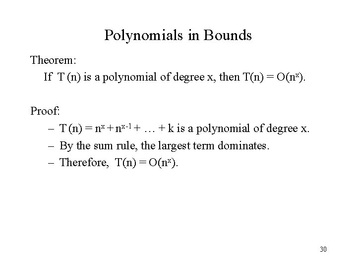
Polynomials in Bounds Theorem: If T (n) is a polynomial of degree x, then T(n) = O(nx). Proof: – T (n) = nx + nx-1 + … + k is a polynomial of degree x. – By the sum rule, the largest term dominates. – Therefore, T(n) = O(nx). 30

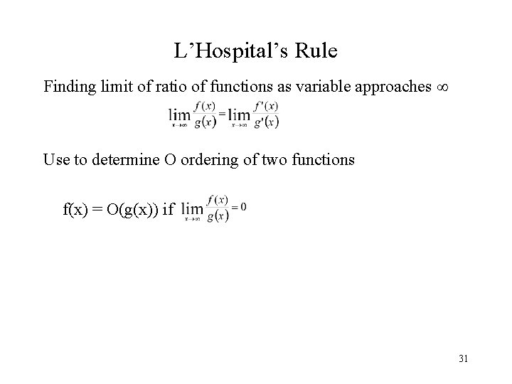
L’Hospital’s Rule Finding limit of ratio of functions as variable approaches Use to determine O ordering of two functions f(x) = O(g(x)) if 31

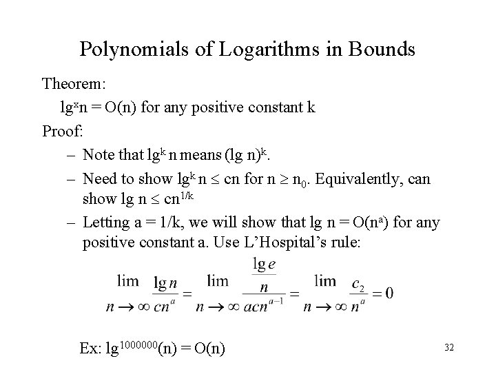
Polynomials of Logarithms in Bounds Theorem: lgxn = O(n) for any positive constant k Proof: – Note that lgk n means (lg n)k. – Need to show lgk n cn for n n 0. Equivalently, can show lg n cn 1/k – Letting a = 1/k, we will show that lg n = O(na) for any positive constant a. Use L’Hospital’s rule: Ex: lg 1000000(n) = O(n) 32

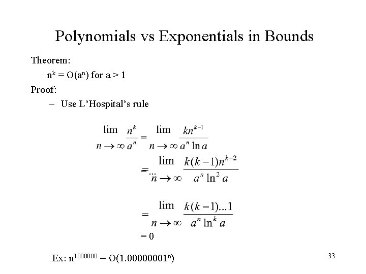
Polynomials vs Exponentials in Bounds Theorem: nk = O(an) for a > 1 Proof: – Use L’Hospital’s rule =. . . =0 Ex: n 1000000 = O(1. 00000001 n) 33

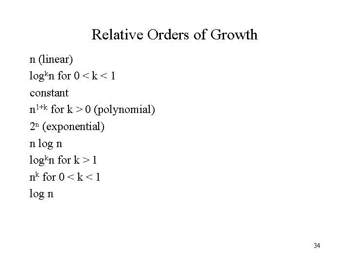
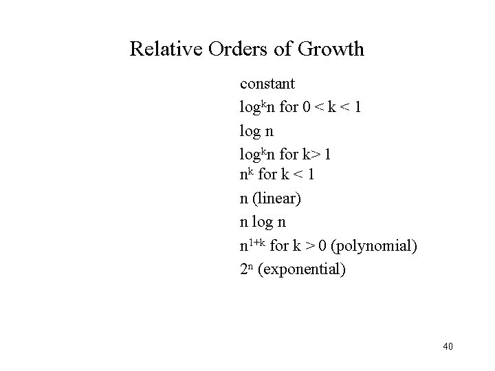
Relative Orders of Growth n (linear) logkn for 0 < k < 1 constant n 1+k for k > 0 (polynomial) 2 n (exponential) n logkn for k > 1 nk for 0 < k < 1 log n 34

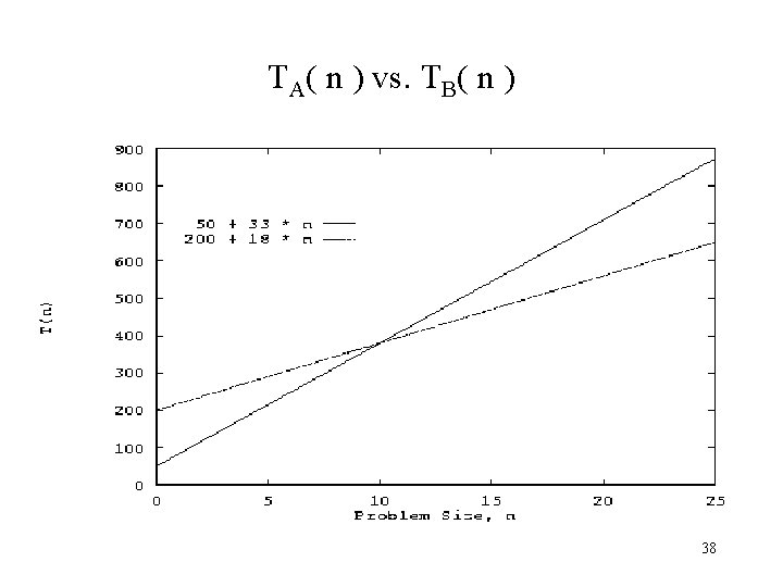
Big-Oh is not the whole story Suppose you have a choice of two approaches to writing a program. Both approaches have the same asymptotic performance (for example, both are O(n lg(n)). Why select one over the other, they're both the same, right? They may not be the same. There is this small matter of the constant of proportionality. Suppose algorithms A and B have the same asymptotic performance, TA(n) = TB(n) = O(g(n)). Now suppose that A does 10 operations for each data item, but algorithm B only does 3. It is reasonable to expect B to be faster than A even though both have the same asymptotic performance. The reason is that asymptotic analysis ignores constants of proportionality. The following slides show a specific example. 35

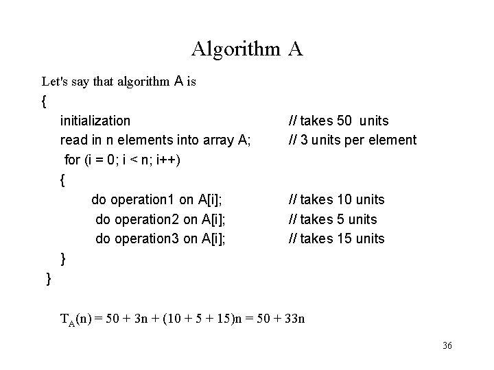
Algorithm A Let's say that algorithm A is { initialization read in n elements into array A; for (i = 0; i < n; i++) { do operation 1 on A[i]; do operation 2 on A[i]; do operation 3 on A[i]; } } // takes 50 units // 3 units per element // takes 10 units // takes 5 units // takes 15 units TA(n) = 50 + 3 n + (10 + 5 + 15)n = 50 + 33 n 36

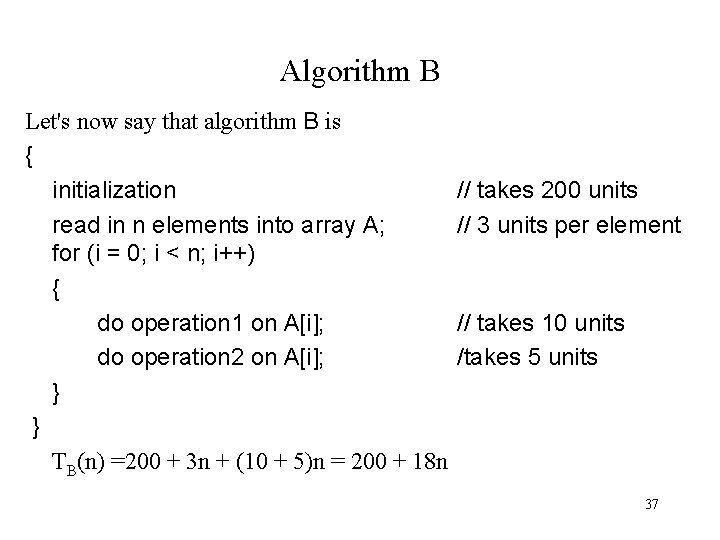
Algorithm B Let's now say that algorithm B is { initialization read in n elements into array A; for (i = 0; i < n; i++) { do operation 1 on A[i]; do operation 2 on A[i]; } } TB(n) =200 + 3 n + (10 + 5)n = 200 + 18 n // takes 200 units // 3 units per element // takes 10 units /takes 5 units 37

TA( n ) vs. TB( n ) 38

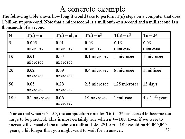
A concrete example The following table shows how long it would take to perform T(n) steps on a computer that does 1 billion steps/second. Note that a microsecond is a millionth of a second a millisecond is a thousandth of a second. N T(n) = nlgn T(n) = n 2 T(n) = n 3 Tn = 2 n 5 0. 005 microsec 0. 01 microsec 0. 03 microsec 0. 13 microsec 0. 03 microsec 10 0. 01 microsec 0. 03 microsec 0. 1 microsec 20 0. 02 microsec 0. 09 microsec 0. 4 microsec 8 microsec 1 millisec 50 0. 05 microsec 0. 28 microsec 2. 5 microsec 125 microsec 13 days 100 0. 1 microsec 0. 66 microsec 10 microsec 1 millisec 4 x 1013 years Notice that when n >= 50, the computation time for T(n) = 2 n has started to become too large to be practical. This is most certainly true when n >= 100. Even if we were to increase the speed of the machine a million-fold, 2 n for n = 100 would be 40, 000 39 years, a bit longer than you might want to wait for an answer.

Relative Orders of Growth constant logkn for 0 < k < 1 log n logkn for k> 1 nk for k < 1 n (linear) n log n n 1+k for k > 0 (polynomial) 2 n (exponential) 40