CMGPDLN Methodological Lecture Day 4 Households Outline Existing

CMGPD-LN Methodological Lecture Day 4 Households

Outline • Existing household variables – Identifiers – Characteristics – Dynamics – Household relationship • Creation of new variables – Use of bysort/egen

Identifiers • HOUSEHOLD_ID – Identifies records associated with a household in the current register • HOUSEHOLD_SEQ – The order of the current household (linghu) within the current household group (yihu) • UNIQUE_HH_ID – Identifies records associated with the same household across different registers – New value assigned at time of household division • Each of the resulting households gets a new, different

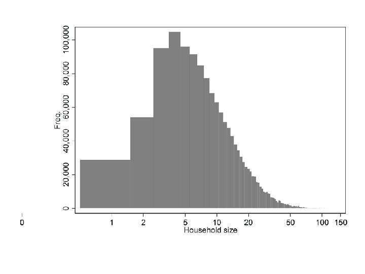
Characteristics • HH_SIZE – Number of living members of the household – Set to missing before 1789 • HH_DIVIDE_NEXT – Number of households in the next register that the members of the current household are associated with. – 1 if no division – 0 if extinction – 2 or more if division – Set to missing before 1789

histogram HH_SIZE if PRESENT & HH_SIZE > 0, width(2) scheme(s 1 mono) fraction ytitle("Proportion of individuals") xtitle("Number of members")

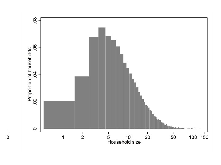
• This isn’t particularly appealing • A log scale on the x axis would help • In STATA, histogram forces fixed width bins, even when the x scale is set to log • We can collapse the data and plot using twoway bar or scatter table HH_SIZE, replace twoway bar table 1 HH_SIZE if HH_SIZE > 0, xscale(log) scheme(s 1 mono) xlabel(0 1 2 5 10 20 50 100 150)

• What if we would like to convert to fractions? • Compute total number of households by summing table 1, then divide each value of table 1 by the total • sum(table 1) returns the sum of table 1 up to the current observation • total[_N] returns the value of total in the last observation drop if HH_SIZE <= 0 generate total = sum(table 1) generate hh_fraction = table 1/total[_N] twoway bar hh_fraction HH_SIZE if HH_SIZE > 0, xscale(log) scheme(s 1 mono) xlabel(0 1 2 5 10 20 50 100 150) ytitle("Proportion of households")

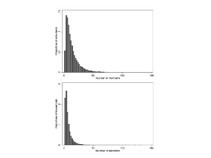
Households as units of analysis • The previous figures all treated individuals as the units of an analysis • Every household was represented as many times as it had members – A household with 100 members would contribute 100 observations • In effect, the figures represent household size as experienced by individuals • Sometimes we would like to treat households as units of analysis – So that each household only contributes one observation per register

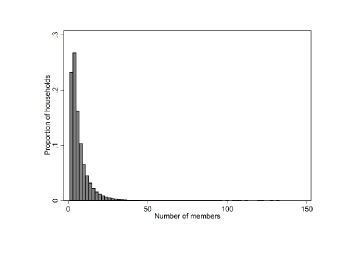
Households as units of analysis • One easy way is to create a flag variable that is set to 1 only for the first observation in each household • Then select based on that flag variable for tabulations etc. • This leaves the original individual level data intact bysort HOUSEHOLD_ID: generate hh_first_record = _n == 1 histogram HH_SIZE if hh_first_record & HH_SIZE > 0, width(2) scheme(s 1 mono) fraction ytitle("Proportion of households") xtitle("Number of members")

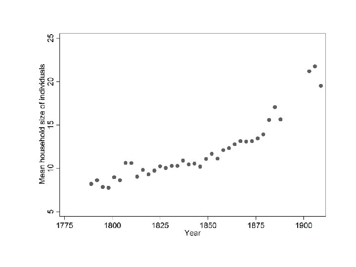
Another approach to plotting trends • We can plot average household size by year of birth without ‘destroying’ the data with TABLE, REPLACE or COLLAPSE bysort YEAR: egen mean_hh_size = mean(HH_SIZE) if HH_SIZE > 0 bysort YEAR: egen first_in_year = _n == 1 twoway scatter mean_hh_size YEAR if first_in_year & YEAR >= 1775, scheme(s 1 mono) ytitle("Mean household size of individuals") xlabel(1775(25)1900)

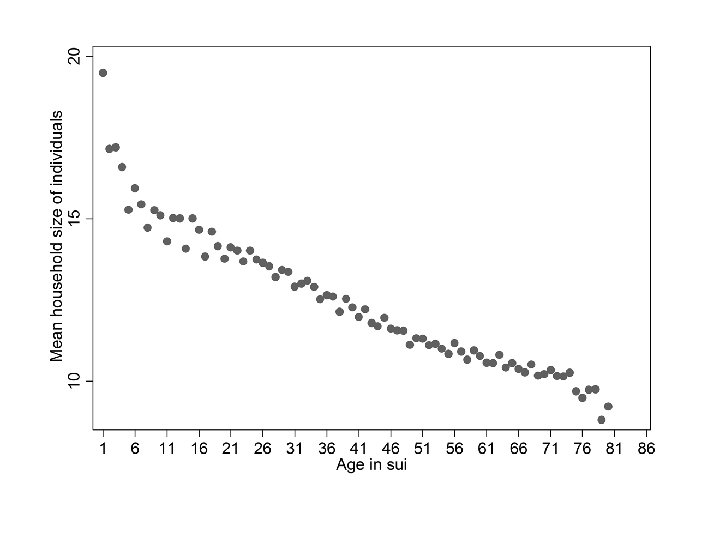
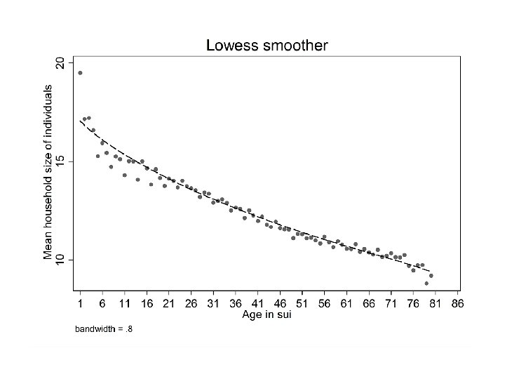
Mean household size of individuals by age keep if AGE_IN_SUI > 0 & SEX == 2 & YEAR >= 1789 & HH_SIZE > 0 bysort AGE_IN_SUI: egen mean_hh_size = mean(HH_SIZE) bysort AGE_IN_SUI: generate first_in_age = _n == 1 twoway scatter mean_hh_size AGE_IN_SUI if first_in_age & AGE_IN_SUI <= 80, scheme(s 1 mono) ytitle("Mean household size of individuals") xlabel(1(5)85) xtitle("Age in sui") lowess mean_hh_size AGE_IN_SUI if first_in_age & AGE_IN_SUI <= 80, scheme(s 1 mono) ytitle("Mean household size of individuals") xlabel(1(5)85) xtitle("Age in sui") msize(small)

Household division Individuals by next register. tab HH_DIVIDE_NEXT if PRESENT & NEXT_3 & HH_DIVIDE_NEXT >= 0 Number of | household in | the next | available | register | Freq. Percent Cum. --------+-----------------1 | 789, 250 94. 98 2 | 33, 000 3. 97 98. 95 3 | 5, 815 0. 70 99. 65 4 | 1, 812 0. 22 99. 87 5 | 383 0. 05 99. 91 6 | 314 0. 04 99. 95 7 | 196 0. 02 99. 98 8 | 34 0. 00 99. 98 9 | 82 0. 01 99. 99 10 | 86 0. 01 100. 00 --------+-----------------Total | 830, 972 100. 00

Household division Households by next register. bysort HOUSEHOLD_ID: generate first_in_hh = _n == 1. tab HH_DIVIDE_NEXT if PRESENT & NEXT_3 & HH_DIVIDE_NEXT >= 0 & first_in_hh Number of | household in | the next | available | register | Freq. Percent Cum. --------+-----------------1 | 117, 317 97. 80 2 | 2, 287 1. 91 99. 71 3 | 272 0. 23 99. 94 4 | 57 0. 05 99. 98 5 | 8 0. 01 99. 99 6 | 7 0. 01 100. 00 7 | 2 0. 00 100. 00 9 | 1 0. 00 100. 00 --------+-----------------Total | 119, 952 100. 00

Household division Example of a simple analysis generate byte DIVISION = HH_DIVIDE_NEXT > 1 generate l_HH_SIZE = ln(HH_SIZE)/ln(1. 1) logit DIVISION HH_SIZE YEAR if HH_SIZE > 0 & NEXT_3 & HH_DIVIDE_NEXT >= 0 & first_in_hh logit DIVISION l_HH_SIZE YEAR if NEXT_3 & HH_DIVIDE_NEXT >= 0 & first_in_hh

. logit DIVISION HH_SIZE YEAR if HH_SIZE > 0 & NEXT_3 & HH_DIVIDE_NEXT >= 0 & first_in_hh Iteration Iteration 0: 1: 2: 3: 4: log log log likelihood likelihood Logistic regression Log likelihood = -14126. 276 = = = -15419. 716 -14310. 848 -14127. 244 -14126. 276 Number of obs LR chi 2(2) Prob > chi 2 Pseudo R 2 = = 132688 2586. 88 0. 0000 0. 0839 ---------------------------------------DIVISION | Coef. Std. Err. z P>|z| [95% Conf. Interval] -------+--------------------------------HH_SIZE |. 0882472. 0016549 53. 32 0. 000. 0850036. 0914908 YEAR | -. 0122989. 0005941 -20. 70 0. 000 -. 0134633 -. 0111345 _cons | 18. 23519 1. 087218 16. 77 0. 000 16. 10428 20. 3661

. logit DIVISION l_HH_SIZE YEAR if NEXT_3 & HH_DIVIDE_NEXT >= 0 & first_in_hh Iteration Iteration 0: 1: 2: 3: 4: 5: log log log likelihood likelihood Logistic regression Log likelihood = -13463. 032 = = = -15419. 716 -13953. 268 -13468. 077 -13463. 036 -13463. 032 Number of obs LR chi 2(2) Prob > chi 2 Pseudo R 2 = = 132688 3913. 37 0. 0000 0. 1269 ---------------------------------------DIVISION | Coef. Std. Err. z P>|z| [95% Conf. Interval] -------+--------------------------------l_HH_SIZE |. 1341566. 0023316 57. 54 0. 000. 1295867. 1387265 YEAR | -. 0130866. 0005775 -22. 66 0. 000 -. 0142185 -. 0119547 _cons | 17. 75924 1. 048066 16. 94 0. 000 15. 70507 19. 81342 ---------------------------------------

Creating household variables • bysort and egen are your friends • Use household_id to group observations of the same household in the same register • Let’s start with a count of the number of live individuals in the household bysort HOUSEHOLD_ID: egen new_hh_size = total(PRESENT). corr HH_SIZE new_hh_size if YEAR >= 1789 (obs=1410354) | HH_SIZE new_hh~e -------+---------HH_SIZE | 1. 0000 new_hh_size | 1. 0000

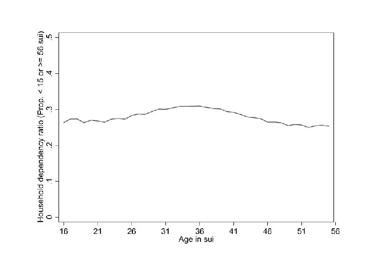
Creating measures of age and sex composition of the household bysort HOUSEHOLD_ID: egen males_1_15 = total(PRESENT & SEX == 2 & AGE_IN_SUI >= 1 & AGE_IN_SUI <= 15) bysort HOUSEHOLD_ID: egen males_16_55 = total(PRESENT & SEX == 2 & AGE_IN_SUI >= 16 & AGE_IN_SUI <= 55) bysort HOUSEHOLD_ID: egen males_56_up = total(PRESENT & SEX == 2 & AGE_IN_SUI >= 56) bysort HOUSEHOLD_ID: egen females_1_15 = total(PRESENT & SEX == 1 & AGE_IN_SUI >= 1 & AGE_IN_SUI <= 15) bysort HOUSEHOLD_ID: egen females_16_55 = total(PRESENT & SEX == 1 & AGE_IN_SUI >= 16 & AGE_IN_SUI <= 55) bysort HOUSEHOLD_ID: egen females_56_up = total(PRESENT & SEX == 1 & AGE_IN_SUI >= 56) generate hh_dependency_ratio = (males_1_15+males 56_up+females_1_15+females 56_up)/HH_SIZE bysort AGE_IN_SUI: generate first_in_age = _n == 1 bysort AGE_IN_SUI: egen mean_hh_dependency_ratio = mean(hh_dependency_ratio) twoway line mean_hh_dependency_ratio AGE_IN_SUI if first_in_age & AGE_IN_SUI >= 16 & AGE_IN_SUI <= 55, scheme(s 1 mono) ylabel(0(0. 1)0. 5) xlabel(16(5)55) ytitle("Household dependency ratio (Prop. < 15 or >= 56 sui)") xtitle("Age in sui")

Numbers of individuals who co-reside with someone who holds a position. bysort HOUSEHOLD_ID: egen position_in_hh = total(PRESENT & HAS_POSITION > 0) . replace position_in_hh = position_in_hh > 0 (49183 real changes made) . tab position_in_hh if PRESENT & YEAR >= 1789 position_in | _hh | Freq. Percent Cum. ------+-----------------0 | 1, 177, 575 90. 23 1 | 87, 517 6. 71 96. 94 2 | 24, 204 1. 85 98. 79 3 | 8, 019 0. 61 99. 41 4 | 4, 893 0. 37 99. 78 5 | 1, 712 0. 13 99. 91 6 | 651 0. 05 99. 96 7 | 241 0. 02 99. 98 8 | 136 0. 01 99. 99 9 | 101 0. 01 100. 00 ------+-----------------Total | 1, 305, 049 100. 00 position_in | _hh | Freq. Percent Cum. ------+-----------------0 | 1, 177, 575 90. 23 1 | 127, 474 9. 77 100. 00 ------+-----------------Total | 1, 305, 049 100. 00