LECTURE DAY 2 Timo Laukkanen What was important

LECTURE DAY 2 Timo Laukkanen

What was important in Lecture 1 • Process Integration/Heat Exchanger Network Synthesis (HENS) is an important step in process design • Energy saving is very often also economically feasible • Energy saving in industry is a major contributor in CO 2 savings in the next 40 years • CC (Composite Curves) • Course arrangements

What is important in Lecture 2 • • • Problem Table Algorithm (PTA) Heat Cascade Grand Composite Curve (GCC) Pinch violations Stream grid Maximum Energy Recovery (MER) Network • Targeting for minimum number of Units

Numerical Method(s) for Energy Targets Problem Table Algorithm, Heat Cascade, Grand Composite Curve

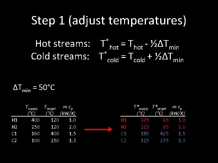
Step 1 (adjust temperatures) Hot streams: T*hot = Thot - ½∆Tmin Cold streams: T*cold = Tcold + ½∆Tmin = 50°C H 1 H 2 C 1 C 2 Tsupply Ttarget m cp (°C) (k. W/K) 400 120 1. 0 250 120 2. 0 160 400 1. 5 100 250 1. 3 H 1 H 2 C 1 C 2 T*supply T*target m cp (°C) (k. W/K) 375 95 1. 0 225 95 2. 0 185 425 1. 5 125 275 1. 3

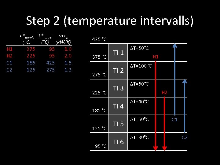
Step 2 (temperature intervalls) H 1 H 2 C 1 C 2 T*supply T*target m cp (°C) (k. W/K) 375 95 1. 0 225 95 2. 0 185 425 1. 5 125 275 1. 3 425 °C 375 °C 225 °C 185 °C 125 °C 95 °C TI 1 TI 2 TI 3 TI 4 TI 5 TI 6 ∆T=50°C H 1 ∆T=100°C ∆T=50°C H 2 ∆T=40°C ∆T=60°C ∆T=30°C C 1 C 2

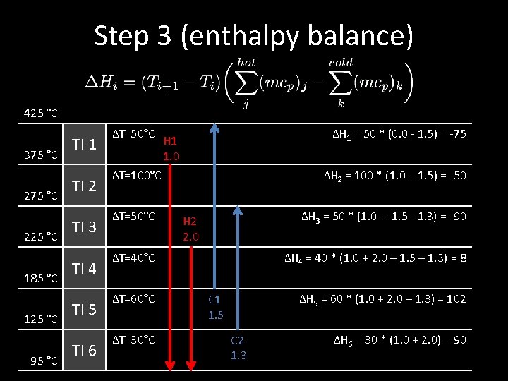
Step 3 (enthalpy balance) 425 °C 375 °C 225 °C 185 °C 125 °C 95 °C TI 1 TI 2 TI 3 TI 4 TI 5 TI 6 ∆T=50°C ∆H 1 = 50 * (0. 0 - 1. 5) = -75 H 1 1. 0 ∆T=100°C ∆T=50°C ∆H 2 = 100 * (1. 0 – 1. 5) = -50 ∆H 3 = 50 * (1. 0 – 1. 5 - 1. 3) = -90 H 2 2. 0 ∆T=40°C ∆T=60°C ∆T=30°C ∆H 4 = 40 * (1. 0 + 2. 0 – 1. 5 – 1. 3) = 8 ∆H 5 = 60 * (1. 0 + 2. 0 – 1. 3) = 102 C 1 1. 5 C 2 1. 3 ∆H 6 = 30 * (1. 0 + 2. 0) = 90

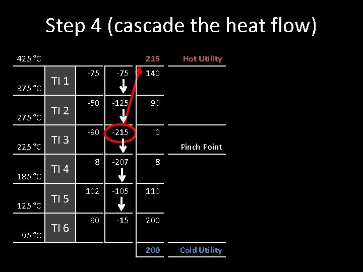
Step 4 (cascade the heat flow) 215 425 °C 375 °C 225 °C 185 °C 125 °C 95 °C TI 1 TI 2 TI 3 TI 4 TI 5 TI 6 -75 140 -50 -125 90 -215 0 Hot Utility Pinch Point 8 -207 8 102 -105 110 90 -15 200 Cold Utility

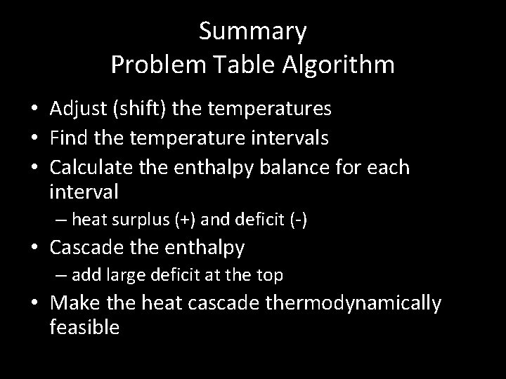
Summary Problem Table Algorithm • Adjust (shift) the temperatures • Find the temperature intervals • Calculate the enthalpy balance for each interval – heat surplus (+) and deficit (-) • Cascade the enthalpy – add large deficit at the top • Make the heat cascade thermodynamically feasible

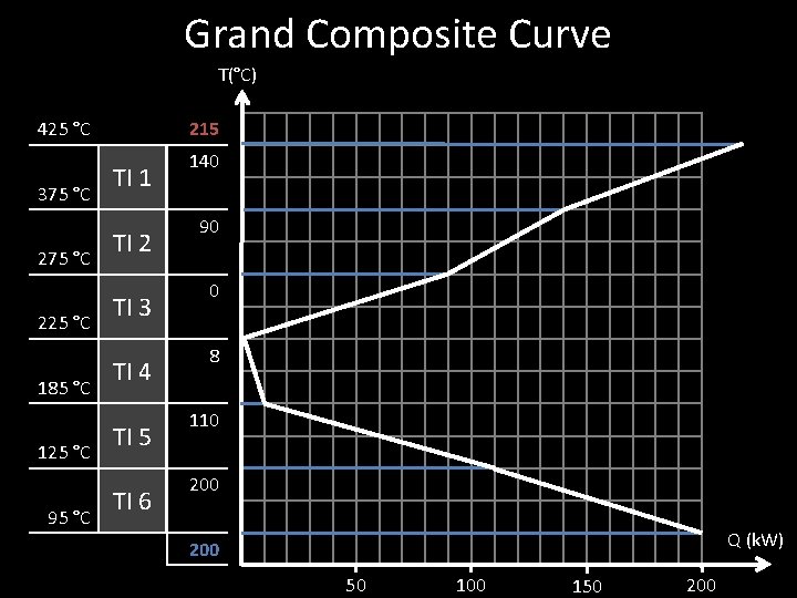
Grand Composite Curve T(°C) 215 425 °C 375 °C 225 °C 185 °C 125 °C 95 °C TI 1 TI 2 TI 3 TI 4 TI 5 TI 6 140 90 0 8 110 200 Q (k. W) 200 50 100 150 200

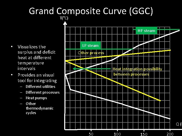
Grand Composite Curve (GGC) T(°C) HP steam • Visualizes the surplus and deficit heat at different temperature intervals • Provides an visual tool for integrating – – LP steam Other process Heat integration possibility between processes Different utilities Different processes Heat pumps Othermodynamic cycles Q (k 50 100 150 200

3 Pinch Rules For Maximum Energy Recovery “Pinch Violations”

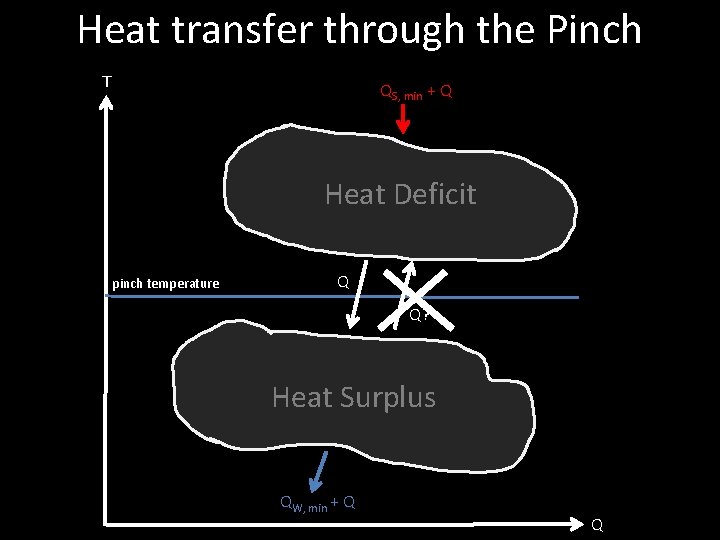
Heat transfer through the Pinch T QS, min + Q Heat Deficit pinch temperature Q Q? Heat Surplus QW, min + Q Q

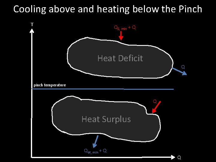
Cooling above and heating below the Pinch T QS, min + Q Heat Deficit Q pinch temperature Q Heat Surplus QW, min + Q Q

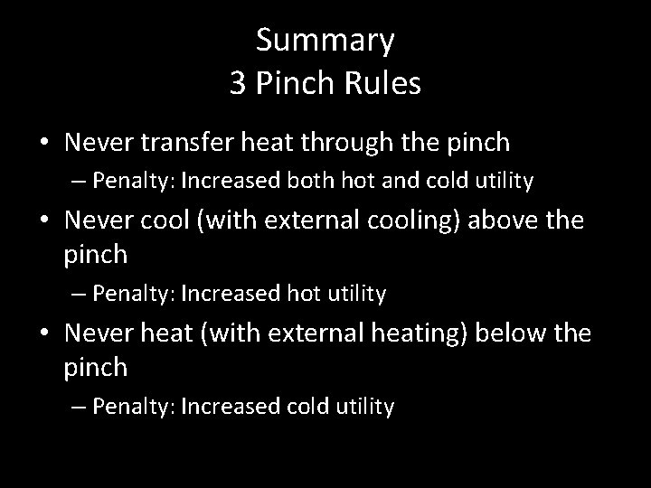
Summary 3 Pinch Rules • Never transfer heat through the pinch – Penalty: Increased both hot and cold utility • Never cool (with external cooling) above the pinch – Penalty: Increased hot utility • Never heat (with external heating) below the pinch – Penalty: Increased cold utility

Heat Exchanger Network Design Stream Grid, MER Network

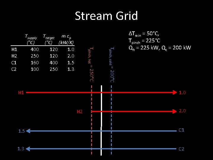
Stream Grid H 1 Tpinch, cold = 200°C H 1 H 2 C 1 C 2 Tpinch, hot = 250°C Tsupply Ttarget m cp (°C) (k. W/K) 400 120 1. 0 250 120 2. 0 160 400 1. 5 100 250 1. 3 ∆Tmin = 50°C, Tpinch = 225°C Qh = 225 k. W, Qc = 200 k. W 1. 0 H 2 2. 0 1. 5 C 1 1. 3 C 2

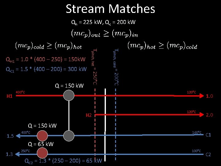
Stream Matches Qh = 225 k. W, Qc = 200 k. W Q = 150 k. W H 1 400°C Tpinch, cold = 200°C QC 1 = 1. 5 * (400 – 200) = 300 k. W Tpinch, hot = 250°C QH 1 = 1. 0 * (400 – 250) = 150 k. W 120°C H 2 120°C 1. 0 2. 0 Q = 150 k. W 1. 5 400°C 160°C C 1 Q = 65 k. W 1. 3 250°C QC 2 = 1. 3 * (250 – 200) = 65 k. W 100°C C 2

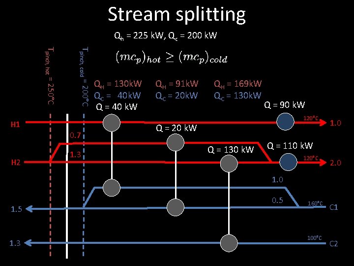
Stream splitting Qh = 225 k. W, Qc = 200 k. W H 2 Tpinch, cold = 200°C Tpinch, hot = 250°C H 1 0. 7 1. 3 QH = 130 k. W QC = 40 k. W Q = 40 k. W QH = 91 k. W QC = 20 k. W QH = 169 k. W QC = 130 k. W Q = 90 k. W 120°C Q = 20 k. W Q = 130 k. W 1. 0 Q = 110 k. W 120°C 2. 0 1. 5 1. 3 0. 5 160°C 100°C C 1 C 2

Summary Stream Grid and MER-Network • Draw the Stream Grid – draw the pinch(es) – draw the streams above and below the pinch • Match streams starting at the pinch – (m cp)out >= (m cp)in – Split streams if necessary • Calculate the heat exchanger duty – Remember hot and cold streams have different pinch temperature!