Chapter 4 Simple Random Sampling SRS SRS SRS

Chapter 4 Simple Random Sampling (SRS)

SRS • SRS – Every sample of size n drawn from a population of size N has the same chance of being selected. • Use table of random numbers (A. 2) or computer software. • Using the table: – Assign every sampling unit a digit – Use table of random numbers to select sample

Example • In a population of N = 450, select a sample of size 10 using the table of random digits. – Starting digit value_______ – Ending digit value_______ – Line number started at _______ – Sample digits selected for sample:

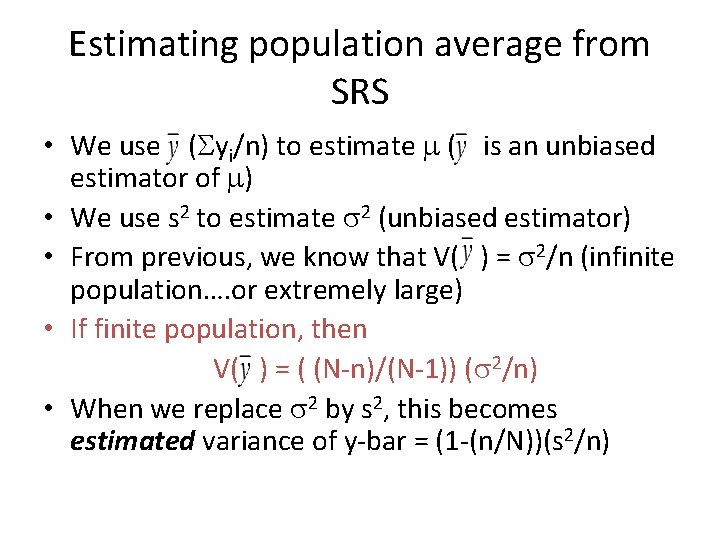
Estimating population average from SRS • We use (Syi/n) to estimate m ( is an unbiased estimator of m) • We use s 2 to estimate s 2 (unbiased estimator) • From previous, we know that V( ) = s 2/n (infinite population…. or extremely large) • If finite population, then V( ) = ( (N-n)/(N-1)) (s 2/n) • When we replace s 2 by s 2, this becomes estimated variance of y-bar = (1 -(n/N))(s 2/n)

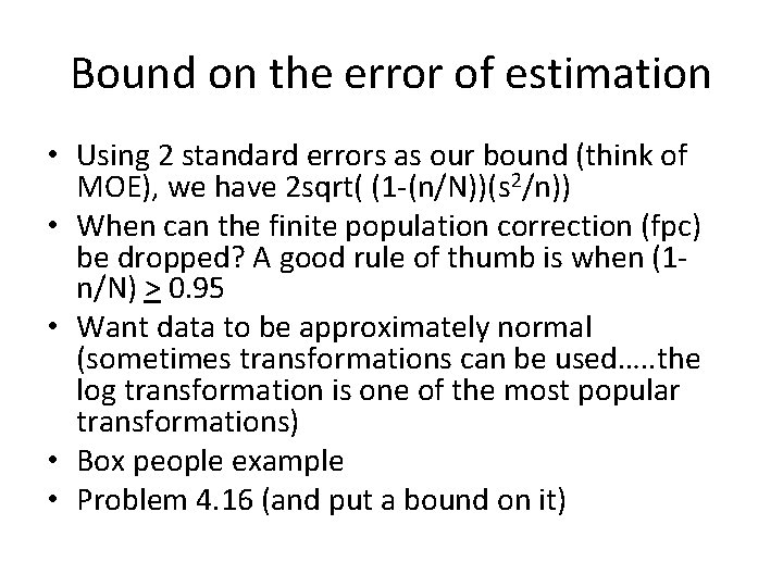
Bound on the error of estimation • Using 2 standard errors as our bound (think of MOE), we have 2 sqrt( (1 -(n/N))(s 2/n)) • When can the finite population correction (fpc) be dropped? A good rule of thumb is when (1 n/N) > 0. 95 • Want data to be approximately normal (sometimes transformations can be used…. . the log transformation is one of the most popular transformations) • Box people example • Problem 4. 16 (and put a bound on it)

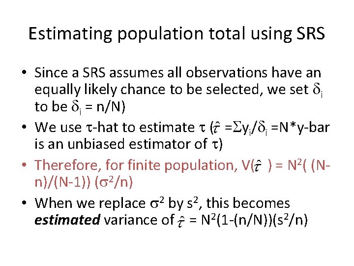
Estimating population total using SRS • Since a SRS assumes all observations have an equally likely chance to be selected, we set di to be di = n/N) • We use t-hat to estimate t ( =Syi/di =N*y-bar is an unbiased estimator of t) • Therefore, for finite population, V( ) = N 2( (Nn)/(N-1)) (s 2/n) • When we replace s 2 by s 2, this becomes estimated variance of = N 2(1 -(n/N))(s 2/n)

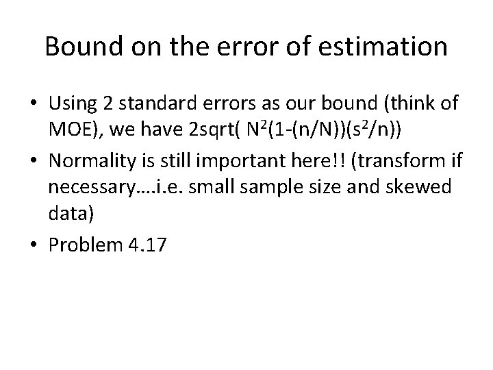
Bound on the error of estimation • Using 2 standard errors as our bound (think of MOE), we have 2 sqrt( N 2(1 -(n/N))(s 2/n)) • Normality is still important here!! (transform if necessary…. i. e. small sample size and skewed data) • Problem 4. 17

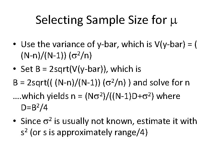
Selecting Sample Size for m • Use the variance of y-bar, which is V(y-bar) = ( (N-n)/(N-1)) (s 2/n) • Set B = 2 sqrt(V(y-bar)), which is B = 2 sqrt(( (N-n)/(N-1)) (s 2/n) ) and solve for n …. which yields n = (Ns 2)/((N-1)D+s 2) where D=B 2/4 • Since s 2 is usually not known, estimate it with s 2 (or s is approximately range/4)

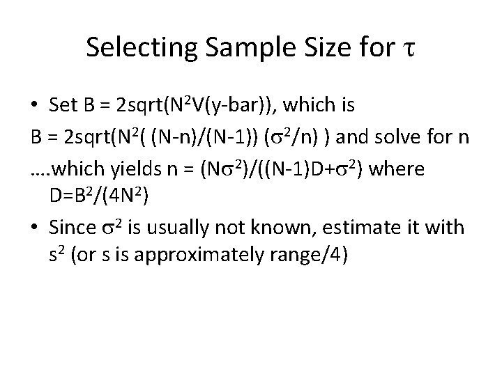
Selecting Sample Size for t • Set B = 2 sqrt(N 2 V(y-bar)), which is B = 2 sqrt(N 2( (N-n)/(N-1)) (s 2/n) ) and solve for n …. which yields n = (Ns 2)/((N-1)D+s 2) where D=B 2/(4 N 2) • Since s 2 is usually not known, estimate it with s 2 (or s is approximately range/4)

Examples • 4. 13, 4. 24, 4. 27, 4. 28

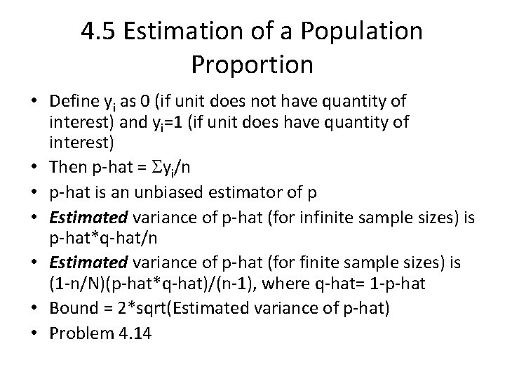
4. 5 Estimation of a Population Proportion • Define yi as 0 (if unit does not have quantity of interest) and yi=1 (if unit does have quantity of interest) • Then p-hat = Syi/n • p-hat is an unbiased estimator of p • Estimated variance of p-hat (for infinite sample sizes) is p-hat*q-hat/n • Estimated variance of p-hat (for finite sample sizes) is (1 -n/N)(p-hat*q-hat)/(n-1), where q-hat= 1 -p-hat • Bound = 2*sqrt(Estimated variance of p-hat) • Problem 4. 14

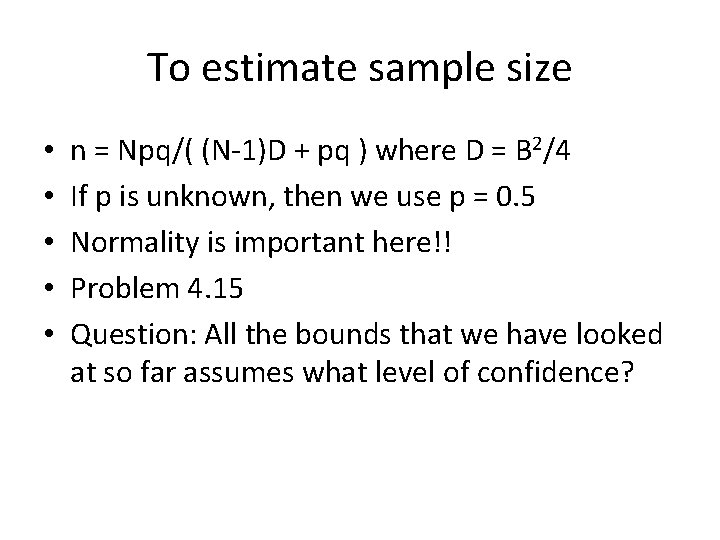
To estimate sample size • • • n = Npq/( (N-1)D + pq ) where D = B 2/4 If p is unknown, then we use p = 0. 5 Normality is important here!! Problem 4. 15 Question: All the bounds that we have looked at so far assumes what level of confidence?

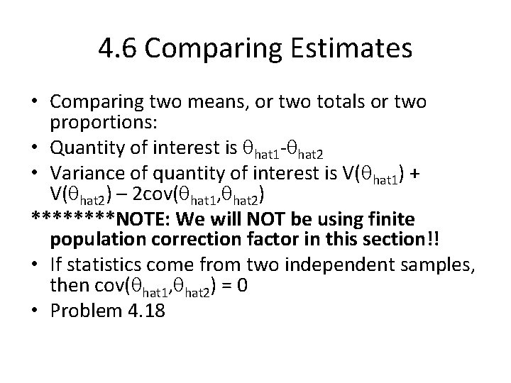
4. 6 Comparing Estimates • Comparing two means, or two totals or two proportions: • Quantity of interest is qhat 1 -qhat 2 • Variance of quantity of interest is V(qhat 1) + V(qhat 2) – 2 cov(qhat 1, qhat 2) ****NOTE: We will NOT be using finite population correction factor in this section!! • If statistics come from two independent samples, then cov(qhat 1, qhat 2) = 0 • Problem 4. 18

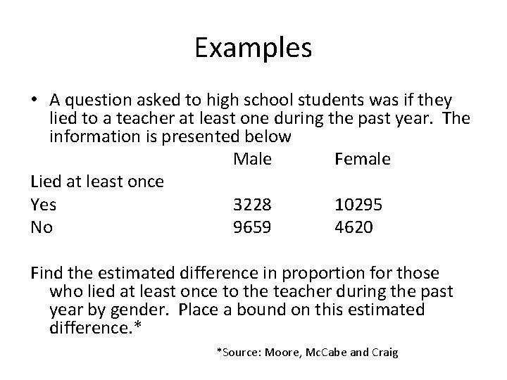
Examples • A question asked to high school students was if they lied to a teacher at least one during the past year. The information is presented below Male Female Lied at least once Yes 3228 10295 No 9659 4620 Find the estimated difference in proportion for those who lied at least once to the teacher during the past year by gender. Place a bound on this estimated difference. * *Source: Moore, Mc. Cabe and Craig

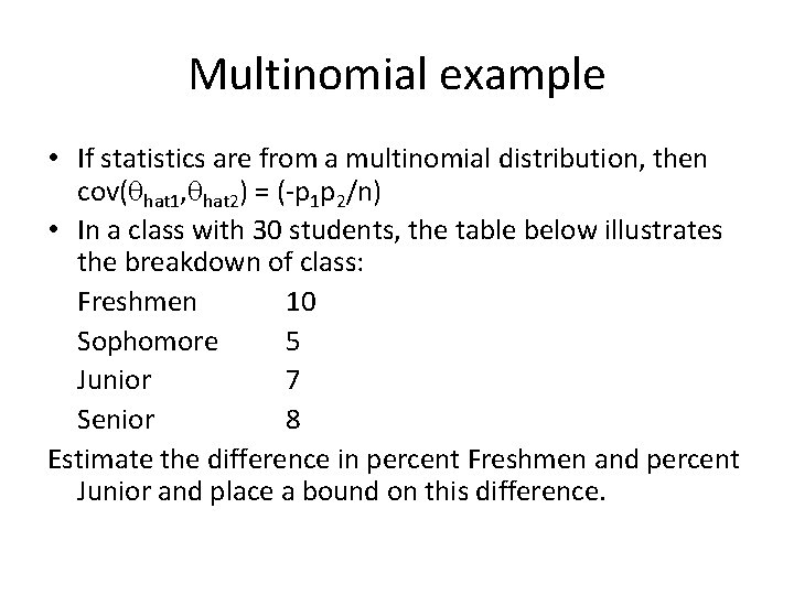
Multinomial example • If statistics are from a multinomial distribution, then cov(qhat 1, qhat 2) = (-p 1 p 2/n) • In a class with 30 students, the table below illustrates the breakdown of class: Freshmen 10 Sophomore 5 Junior 7 Senior 8 Estimate the difference in percent Freshmen and percent Junior and place a bound on this difference.