A RealTime Water Quality Monitoring Network for Investigating

A Real-Time Water Quality Monitoring Network for Investigating the Strengths and Weaknesses of Existing Monitoring Techniques David K. Stevens 1, Jeffery S. Horsburgh 1, Nancy Mesner 2 Amber Spackman 1 2 Dept. 1 Utah Water Research Laboratory of Aquatic, Watershed, and Earth Resources Utah State University, Logan, UT

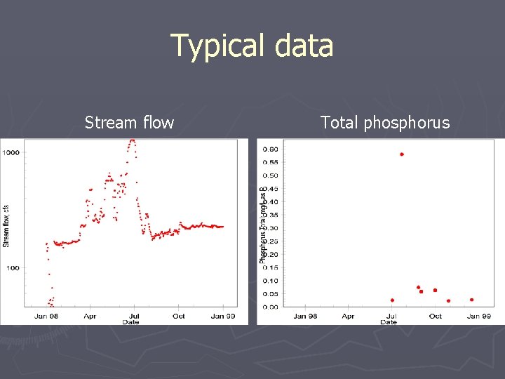
The Interesting Questions ► Is traditional monitoring adequate to characterize natural or anthropogenic variability in flow and total phosphorus concentrations? ► Do in stream monitoring data used in typical TMDLs focus too much on point source loads when intermittent or infrequent nonpoint source loads may be important?

Current project ► Continuous water quality monitoring effort in the Little Bear River of Northern Utah § continuous flow/water quality paired with periodic and storm event sampling § designed to evaluate the strengths and weaknesses of each of the water quality monitoring techniques § focus on correlating the results of high frequency turbidity, oxygen, temperature, conductance and p. H (possible others) monitoring with those of traditional sampling

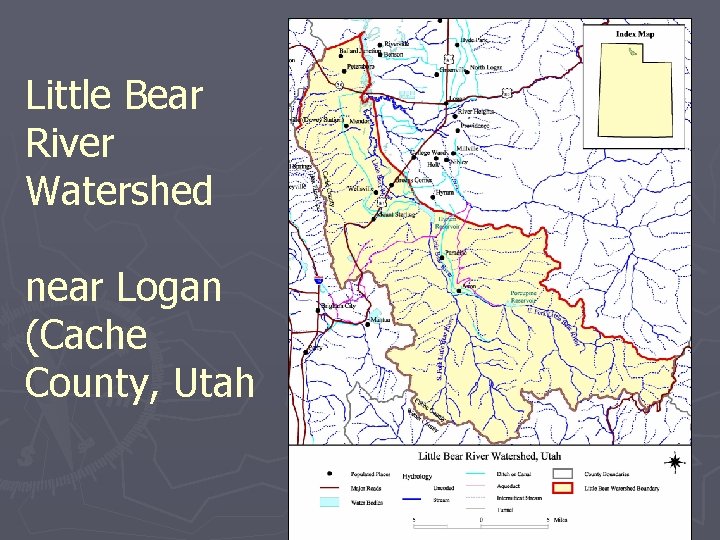
Little Bear River Watershed near Logan (Cache County, Utah

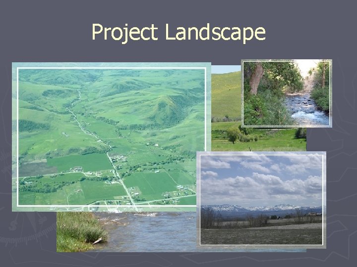
Project Landscape

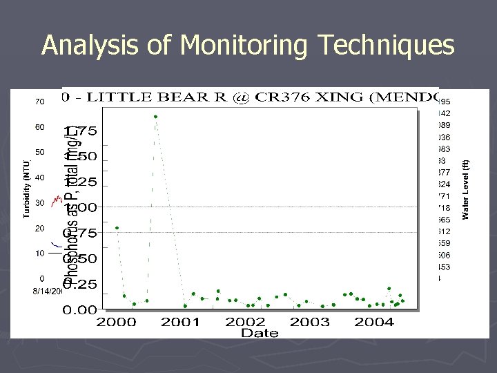
Typical data Stream flow Total phosphorus

Analysis of Monitoring Techniques

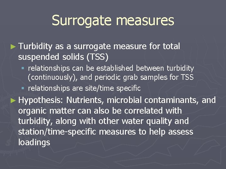
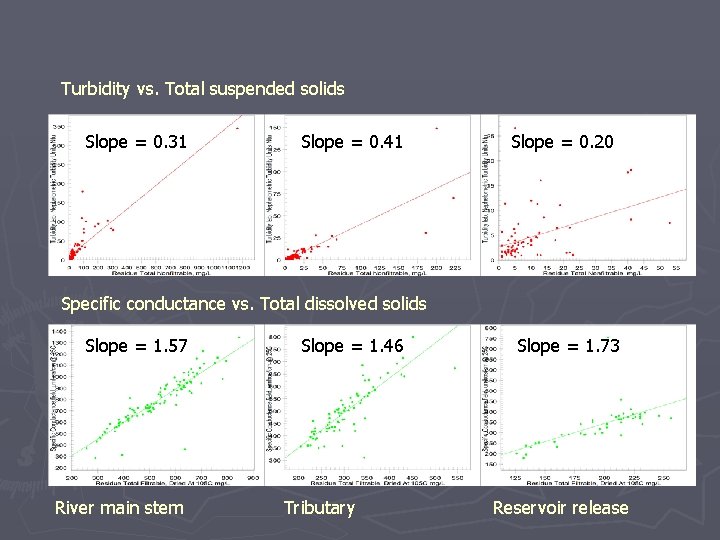
Surrogate measures ► Turbidity as a surrogate measure for total suspended solids (TSS) § relationships can be established between turbidity (continuously), and periodic grab samples for TSS § relationships are site/time specific ► Hypothesis: Nutrients, microbial contaminants, and organic matter can also be correlated with turbidity, along with other water quality and station/time-specific measures to help assess loadings

Turbidity vs. Total suspended solids Slope = 0. 31 Slope = 0. 41 Slope = 0. 20 Specific conductance vs. Total dissolved solids Slope = 1. 57 River main stem Slope = 1. 46 Tributary Slope = 1. 73 Reservoir release

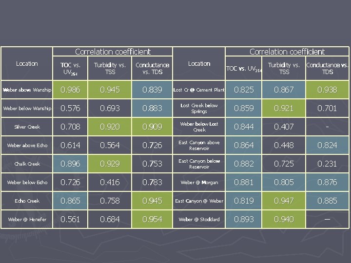
Correlation coefficient Location TOC vs. UV 254 Turbidity vs. TSS Conductance vs. TDS Location Weber above Wanship 0. 986 0. 945 0. 839 Weber below Wanship 0. 576 0. 693 Silver Creek 0. 708 Weber above Echo TOC vs. UV 254 Turbidity vs. TSS Conductance vs. TDS Lost Cr @ Cement Plant 0. 825 0. 867 0. 938 0. 883 Lost Creek below Springs 0. 859 0. 921 0. 701 0. 920 0. 909 Weber below Lost Creek 0. 844 0. 407 - 0. 614 0. 564 0. 726 East Canyon above Reservoir 0. 864 0. 448 0. 824 Chalk Creek 0. 896 0. 929 0. 753 East Canyon below Reservoir 0. 882 0. 725 0. 231 Weber below Echo 0. 726 0. 416 0. 783 Weber @ Morgan 0. 881 0. 805 0. 876 Echo Creek 0. 865 0. 758 0. 945 East Canyon @ Weber 0. 819 0. 947 0. 885 Weber @ Henefer 0. 561 0. 684 0. 954 Weber @ Stoddard 0. 893 0. 940 --

Bayesian networks ► Probabilistic network models § graphical representation § relationships among variables exogenous, ► state, and ►system ► ► Directed acyclic graph § causal structure of variables § conditional probability distributions

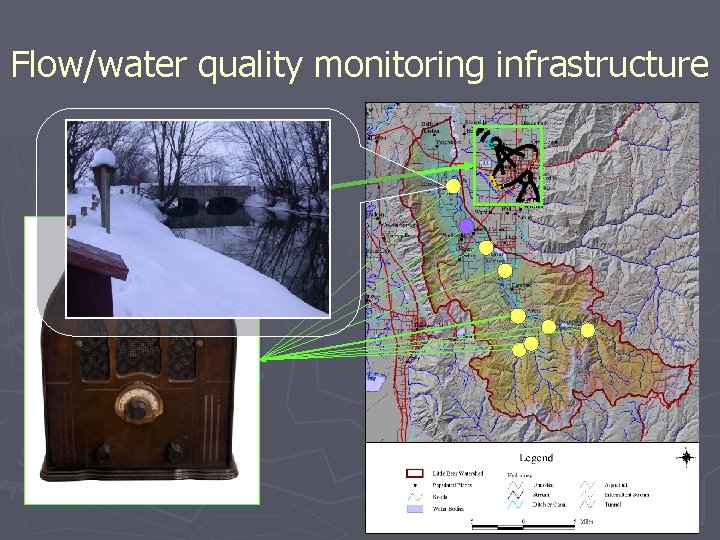
Little Bear River Sampling Program Continuous Monitoring Equipment ► Stage recording devices to estimate discharge sensors to monitor water quality http: //www. campbellsci. com ► Turbidity ► Dataloggers telemetry equipment http: //www. ftsinc. com/ and http: //www. campbellsci. com

Flow/water quality monitoring infrastructure

Continuous Monitoring Data Little Bear River Near Paradise Storm Event

Monitoring infrastructure …

Little Bear River Sampling Program Periodic Baseline Sampling ► Continuous flow, temp. , D. O. , p. H, Spec. cond. , turbidity ► Field samples collected weekly or bi-weekly depending on the time of year and analyzed for: § Nutrients § Total suspended solids § Total dissolved solids ► Simultaneous spot checks of turbidity with a portable field meter ► Establish relationships between total phosphorus, total suspended, dissolved solids, turbidity, flow, time, watershed characteristics, others

… Starting this fall ► Monitoring § Add four continuous climate stations § Add six new continuous water quality monitoring stations ► Analysis § Construct time series of estimates for constituents § Study the high frequency patterns of estimated nutrient loading ► Cyberinfrastructure improvement (session K 1 -2, tomorrow afternoon)

What do we gain? ► Greatly reduced uncertainty in flows and concentrations at a reasonable cost § Use large quantities of relatively low cost (read: less precise) data rather than small(er) quantities of expensive (more precise) data ► Potential characterization of pollutant loading down to an hourly scale with uncertainty estimates via Bayes networks?

Do in-stream monitoring data used in TMDLs focus too much on relatively steady point source loads when intermittent or infrequent nonpoint source loads are important? ► Is it worth while for a POTW to install monitoring equipment downstream of a discharge to better characterize the full spectrum of loading in the stream? – as opposed to ► Traditional ambient monitoring that may only characterize the times when loading in the stream is dominated by WWTP discharges, e. g. East Canyon Creek, Park City, UT - Up to 50 % of the flow at times is WWTP discharge, but 50% of annual total phosphorus load may occur during one storm event

Where are we headed? ► Rigorously explore the relationships between the surrogates and the parameters of interest ► Explore spatial/temporal influences on these relationships ► Analyze the significance of storm event loads vs. base flow loads ► Back next NWQMC

Conclusions ► Status of monitoring network § First two stations established August ’ 05 § Field sampling initiated March ’ 06 – data just now becoming available § Reliability high with ‘graduate student’ maintenance

Conclusions ► Future § Dramatically increase amount of data ► flow, continuous, field water ► climate (four new stations) quality § Externalities ► update/improve resolution of land use/land cover ► update irrigation practice information (diversions, return flow, etc. ) ► complete data acquisition for nutrient management pactices/BMP § Long term ► help provide information for development of hydrologic/environmental observatories with NSF/EPA support

Acknowledgements ► USDA/CEAP ► State of Utah, Division of Water Quality ► Natural Resources Conservation Service ► USU Water Initiative ► Utah Water Research Laboratory ► National Science Foundation (hydrologic/environmental observatories)

Abstract ► Traditional water quality monitoring approaches § grab and/or composite samples § supporting in-stream measurements of temperature, dissolved oxygen, p. H, and specific conductance § monthly, bi-weekly, or even weekly frequency § inadequate to the variability in pollutant concentrations § underestimation of pollutant loads and a greater focus on steady point source loading when intermittent or infrequent nonpoint source loads are important but not characterized by grab samples.

Objective 1 ► Construct time series of estimates for constituents § Bayesian Network models ► real time estimation of constituent fluxes and concentrations conditional upon surrogate measurements. § Uncertainty associated with Bayesian estimates of constituent concentration and loading ► can be used to optimize the collection field samples

Objective 2 ► Study the high frequency patterns of estimated nutrient loading § § § High frequency information more effective for quantifying the relationships between constituent concentrations and watershed attributes and management practices Significant nutrient fluxes are associated with episodic events that can only be quantified through high frequency sampling. Nutrient loading estimates to quantify the probability distributions to Bayesian Network models - smaller uncertainty

Objective 3 ► Cyberinfrastructure § Seamless, two-way linkages between sensors and ►a central observations database that stores and archives the observations; ► models or data analysis software that use the data; ► connected via a telemetry system; ► interfaced with a central hydrologic observations database via data filters and QA/QC. § Data are immediately available for analysis, modeling, and decision making. § Bayesian Network outputs to trigger the collection of field samples to estimate loads

Observations infrastructure ► Currently monitoring § stream flow and turbidity at high frequency at two sites relayed via radio frequency transmission to a base station at the Utah Water Research Laboratory. § routine and episodic grab sampling at these two sites ► This fall § instrument six additional sites, each of which is an historic USGS stream flow gauging location § continuously monitor stream flow, turbidity, dissolved oxygen, specific conductance, and water temperature § expand field/automatic sampling efforts to new sites

Little Bear River Sampling Program Storm Event Sampling ► Automated sampling of storm events ► Triggered by precipitation ► Characterize the system response ► Rise and fall of storm hydrograph