3 2 Scaled Random Walks 3 2 Scaled


+1")


 integer s t")


 (t) is mtgle. Linearity of conditional expectations 16")


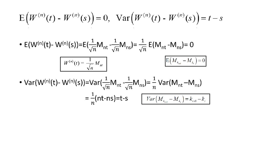
(t)- W(n)(s))=0 Var(W(n)(t)- W(n)(s))=t-s S=0 E(W(n)(t))=0 Var(W(n)(t))=t N(0,")
 • Asked to compute")
 • Outline of proof: 藉由動差生成函數(MGF)的唯一性來判斷r. v. 屬於何種分配")
 Normal density N(ut, t) =1")

(0. 25)~N(0, 0. 25)")
- Slides: 26
3. 2 Scaled Random Walks 黃于珊
3. 2 Scaled Random Walks • Properties of symmetric random walk • Increments • Martingale • Quadratic Variation
3. 2. 1 Symmetric Random Walk Toss a fair coin repeatedly • With each toss, it either steps up one unit or down one unit, and each of the two probabilities is equally likely • Define =0, is a symmetric random walk 3
3. 2. 2 Increments of the Symmetric Random Walk • A random walk has independent increments • If we choose nonnegative integers 0= , are independent
3. 2. 2 Increments of the Symmetric Random Walk is called an increment of the random walk • ki+1=4 k 1 k 2 3= ki ki+1 =5 • Increments over nonoverlapping time intervals are indep. because they depend on different coin tosses • E( )=0 • Var( )= M 5 -M 3=X 4+X 5
Proof of
Proof of =ki+1 -(ki+1)+1
3. 2. 3 Martingale Property for the Symmetric Random Walk • Choose nonnegative integers k < l , then, Linearity of conditional expectations Mk為Fk可測 • 在Fk資訊集合的情況下Ml的期望值為Mk 8
3. 2. 4 Quadratic Variation of the Symmetric Random Walk • The quadratic variation up to time k is defined to be (3. 2. 6) One-step increments Mj-Mj-1=Xj, Xj 2=1 • Note : .This is computed path-by-path .by taking all the one-step increments along that path, squaring these increments, and then summing them 9
How to compute the 10
3. 2. 5 Scaled Symmetric Random Walk • (3. 2. 7) integer s t u 11
Property of Scaled Random Walk because they depend on different coin tosses
The martingale property for scaled random walk ØLet be given, and decompose as ØIf s and t are chosen so that ns and nt are integers 15
Prove W(n) (t) is mtgle. Linearity of conditional expectations 16
Quadratic variation of the scaled random walk 每段時間的增量 平方後加總 Mj-Mj-1=Xj , Xj 2=1 進行計算的 時間長度 17
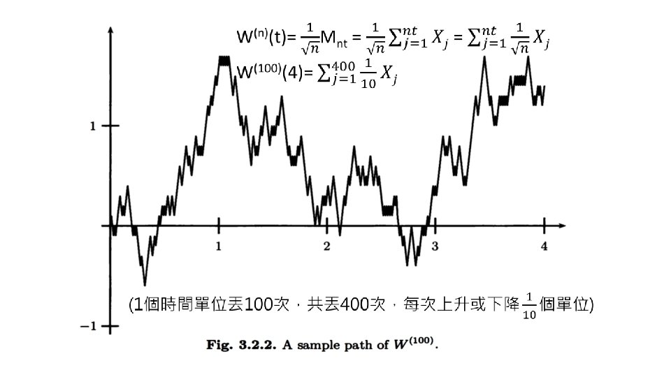
3. 2. 6 Limiting Distribution of the Scaled Random Walk • fixed a sequence of coin tosses and drawn the path of the resulting process as time t varies Figure 3. 2. 2 • Fix t and consider the set of all possible paths evaluated at that time t ØSet t = 0. 25 and consider the set of possible values of ØM 25 can take any odd integer (丟奇數次 奇H, 偶T 偶H, 奇T ) between -25 and 25 W(100)(0. 25) can take any of the values -2. 5, -2. 3, …, -0. 3, -0. 1, 0. 3, … 2. 3, 2. 5 ØIn order for to take value 0. 1, we must get 13 H and 12 T in the 25 coin tosses. The probability of this is 18
the distribution of is nearly normal E(W(n)(t)- W(n)(s))=0 Var(W(n)(t)- W(n)(s))=t-s S=0 E(W(n)(t))=0 Var(W(n)(t))=t N(0, 0. 25) 0. 2 The bar has width 0. 2, its height must be 0. 1555 / 0. 2 = 0. 7775 19
Approximate the integral • Given a continuous bounded function g(x) • Asked to compute • We can obtain a good approximation by multiplying g(x) by the normal density and integrating (3. 2. 12) • The Central Limit Theorem asserts that the approximation in (3. 2. 12) is valid 20
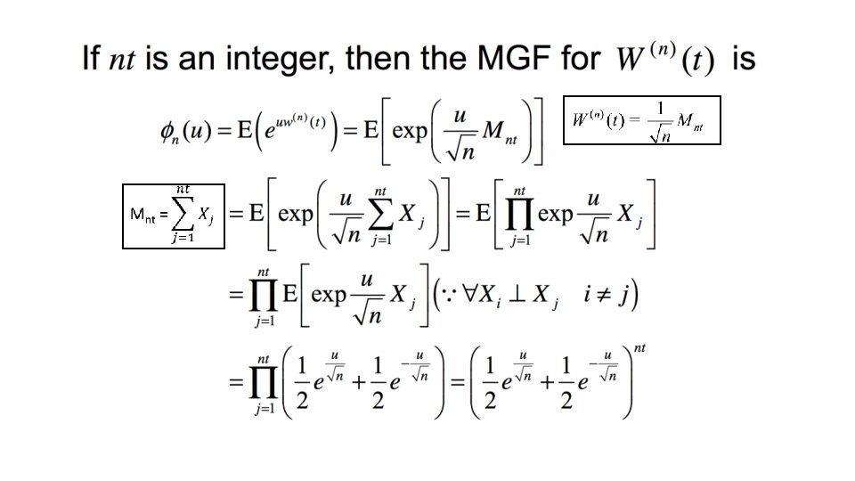
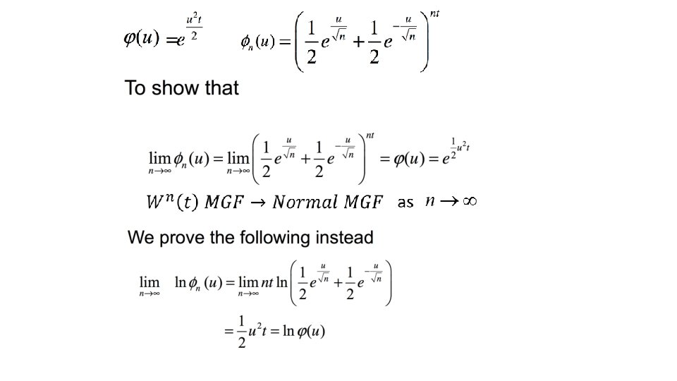
Theorem 3. 2. 1 (Central Limit Theorem) • Outline of proof: 藉由動差生成函數(MGF)的唯一性來判斷r. v. 屬於何種分配 as as 21
X~N(0, t) Normal density N(ut, t) =1
-ux
W(100)(0. 25)~N(0, 0. 25)