10 Market microstructure inventory models 10 1 Introduction

10. Market microstructure: inventory models 10. 1 Introduction Dealers must maintain inventory on both sides of the market. Inventory risk: buy order flows and sell order flows are not balanced. Bid/ask spread compensates inventory risk. Inventory models - risk-neutral: Garman (1976), Amihud & Mendelson (1980) - with risk aversion: Stoll (1978) Walrasian equilibrium: price is determined by equilibrium between supply and demand 1

10. Market microstructure: inventory models 2

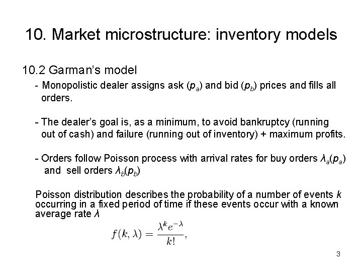
10. Market microstructure: inventory models 10. 2 Garman’s model - Monopolistic dealer assigns ask (pa) and bid (pb) prices and fills all orders. - The dealer’s goal is, as a minimum, to avoid bankruptcy (running out of cash) and failure (running out of inventory) + maximum profits. - Orders follow Poisson process with arrival rates for buy orders λa(pa) and sell orders λb(pb) Poisson distribution describes the probability of a number of events k occurring in a fixed period of time if these events occur with a known average rate λ 3

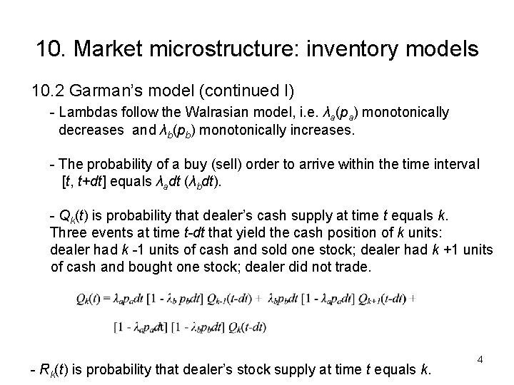
10. Market microstructure: inventory models 10. 2 Garman’s model (continued I) - Lambdas follow the Walrasian model, i. e. λa(pa) monotonically decreases and λb(pb) monotonically increases. - The probability of a buy (sell) order to arrive within the time interval [t, t+dt] equals λadt (λbdt). - Qk(t) is probability that dealer’s cash supply at time t equals k. Three events at time t-dt that yield the cash position of k units: dealer had k -1 units of cash and sold one stock; dealer had k +1 units of cash and bought one stock; dealer did not trade. - Rk(t) is probability that dealer’s stock supply at time t equals k. 4

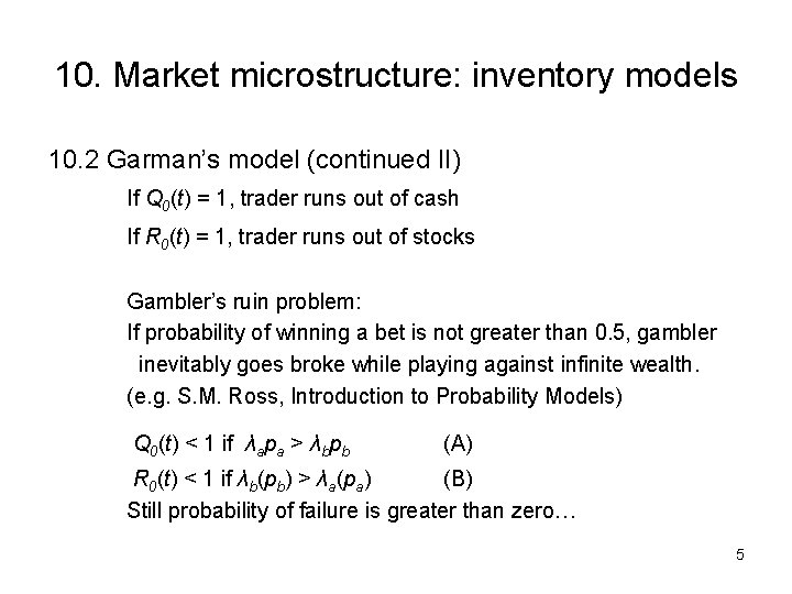
10. Market microstructure: inventory models 10. 2 Garman’s model (continued II) If Q 0(t) = 1, trader runs out of cash If R 0(t) = 1, trader runs out of stocks Gambler’s ruin problem: If probability of winning a bet is not greater than 0. 5, gambler inevitably goes broke while playing against infinite wealth. (e. g. S. M. Ross, Introduction to Probability Models) Q 0(t) < 1 if λapa > λbpb (A) R 0(t) < 1 if λb(pb) > λa(pa) (B) Still probability of failure is greater than zero… 5

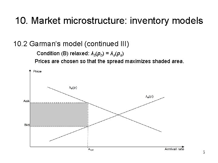
10. Market microstructure: inventory models 10. 2 Garman’s model (continued III) Condition (B) relaxed: λb(pb) = λa(pa) Prices are chosen so that the spread maximizes shaded area. 6

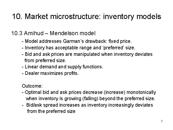
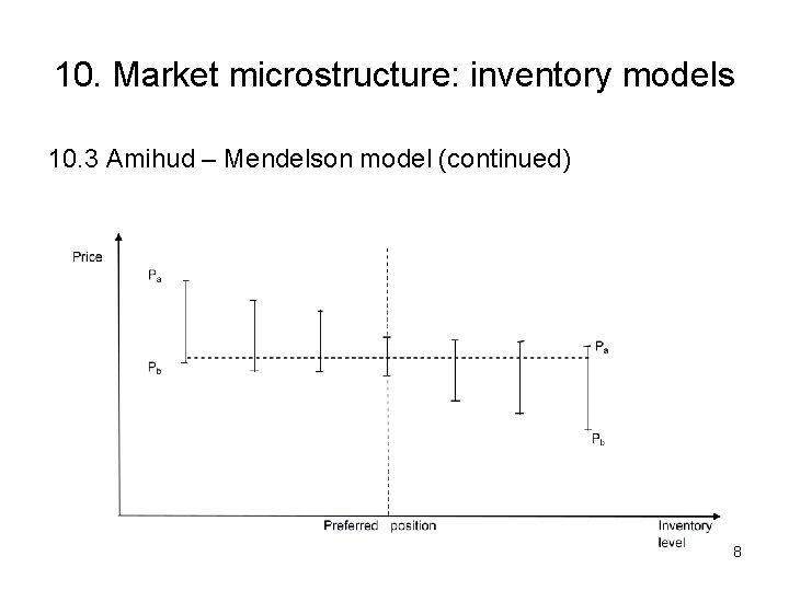
10. Market microstructure: inventory models 10. 3 Amihud – Mendelson model - Model addresses Garman’s drawback: fixed price. - Inventory has acceptable range and ‘preferred’ size. - Bid and ask prices are manipulated when inventory deviates from preferred size. - Linear demand supply functions. - Dealer maximizes profits. Outcome: - Optimal bid and ask prices decrease (increase) monotonically when inventory is growing (falling) beyond the preferred size. - Bid/ask spread increases as inventory increasingly deviates from the preferred size 7

10. Market microstructure: inventory models 10. 3 Amihud – Mendelson model (continued) 8

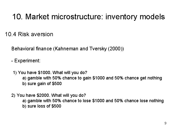
10. Market microstructure: inventory models 10. 4 Risk aversion Behavioral finance (Kahneman and Tversky (2000)) - Experiment: 1) You have $1000. What will you do? a) gamble with 50% chance to gain $1000 and 50% chance get nothing b) sure gain of $500 2) You have $2000. What will you do? a) gamble with 50% chance to lose $1000 and 50% chance lose nothing b) sure loss of $500 9

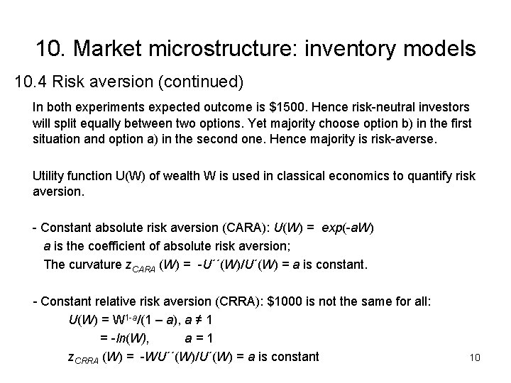
10. Market microstructure: inventory models 10. 4 Risk aversion (continued) In both experiments expected outcome is $1500. Hence risk-neutral investors will split equally between two options. Yet majority choose option b) in the first situation and option a) in the second one. Hence majority is risk-averse. Utility function U(W) of wealth W is used in classical economics to quantify risk aversion. - Constant absolute risk aversion (CARA): U(W) = exp(-a. W) a is the coefficient of absolute risk aversion; The curvature z. CARA (W) = -U´´(W)/U´(W) = a is constant. - Constant relative risk aversion (CRRA): $1000 is not the same for all: U(W) = W 1 -a/(1 – a), a ≠ 1 = -ln(W), a=1 z. CRRA (W) = -WU´´(W)/U´(W) = a is constant 10

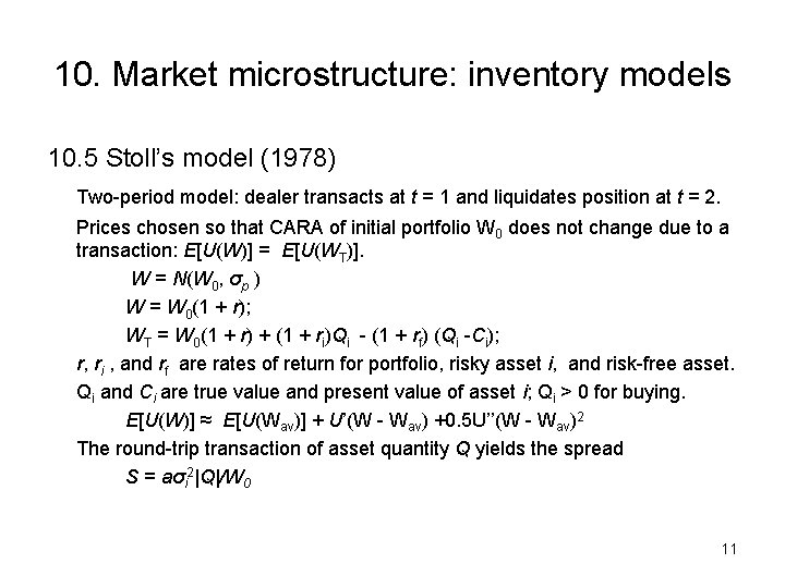
10. Market microstructure: inventory models 10. 5 Stoll’s model (1978) Two-period model: dealer transacts at t = 1 and liquidates position at t = 2. Prices chosen so that CARA of initial portfolio W 0 does not change due to a transaction: E[U(W)] = E[U(WT)]. W = N(W 0, σp ) W = W 0(1 + r); WT = W 0(1 + r) + (1 + ri)Qi - (1 + rf) (Qi -Ci); r, ri , and rf are rates of return for portfolio, risky asset i, and risk-free asset. Qi and Ci are true value and present value of asset i; Qi > 0 for buying. E[U(W)] ≈ E[U(Wav)] + U’(W - Wav) +0. 5 U’’(W - Wav)2 The round-trip transaction of asset quantity Q yields the spread S = aσi 2|Q|/W 0 11

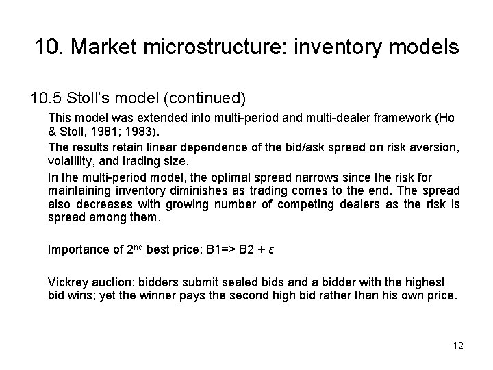
10. Market microstructure: inventory models 10. 5 Stoll’s model (continued) This model was extended into multi-period and multi-dealer framework (Ho & Stoll, 1981; 1983). The results retain linear dependence of the bid/ask spread on risk aversion, volatility, and trading size. In the multi-period model, the optimal spread narrows since the risk for maintaining inventory diminishes as trading comes to the end. The spread also decreases with growing number of competing dealers as the risk is spread among them. Importance of 2 nd best price: B 1=> B 2 + ε Vickrey auction: bidders submit sealed bids and a bidder with the highest bid wins; yet the winner pays the second high bid rather than his own price. 12

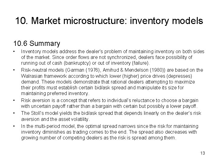
10. Market microstructure: inventory models 10. 6 Summary • • • Inventory models address the dealer’s problem of maintaining inventory on both sides of the market. Since order flows are not synchronized, dealers face possibility of running out of cash (bankruptcy) or out of inventory (failure). Risk-neutral models (Garman (1976), Amihud & Mendelson (1980)) are based on the Walrasian framework according to which lower (higher) price drives (depresses) demand. These models demonstrate that rational dealers attempting to maximize their profits must establish certain bid/ask spread and manipulate its size for maintaining preferred inventory. Risk aversion is a concept that refers to individual’s reluctance to choose a bargain with uncertain payoff rather than a bargain with certain but possibly a lower payoff. The Stoll’s model yields the bid/ask spread that depends linearly on the dealer’s risk aversion and the asset volatility. In the multi-period model, the optimal spread narrows since the risk for maintaining inventory diminishes as trading comes to the end. The spread also decreases with growing number of competing dealers as the risk is spread among them. 13