Withdrawal period calculation conforming to Japanese guidelines 2019

Withdrawal period calculation conforming to Japanese guidelines 2019. 11. 20 VOF in Akishima TOKYO Kaoru Eguchi National Veterinary Assay Laboratory JMAFF 1

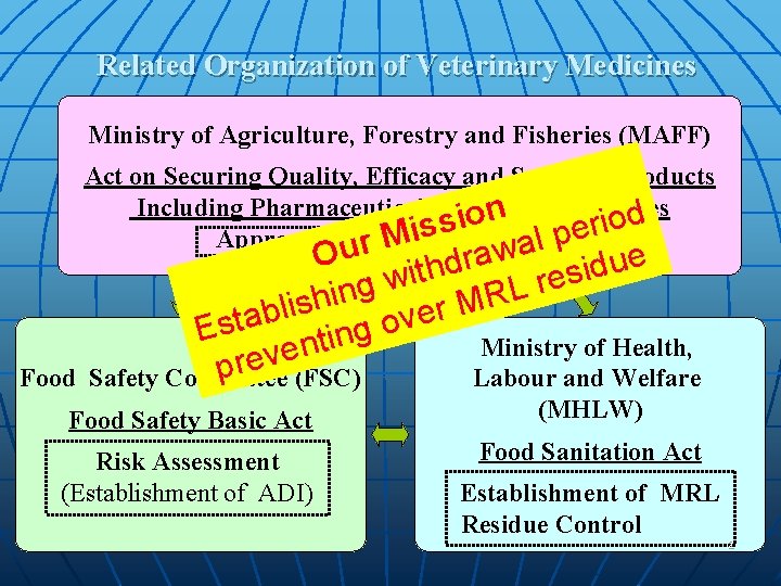
Related Organization of Veterinary Medicines Ministry of Agriculture, Forestry and Fisheries (MAFF) Act on Securing Quality, Efficacy and Safety of Products Including Pharmaceuticals and Medical Devices n d o i s r s e i Approval of Veterinary medicine r. M al p Food Ou ithdraw e u d i s e w r g L n i R h s M i l r b a ve t o s E g n i t Ministry of Health, n e v e r p Labour and Welfare Safety Committee (FSC) Food Safety Basic Act (MHLW) Risk Assessment (Establishment of ADI) Food Sanitation Act Establishment of MRL Residue Control 2

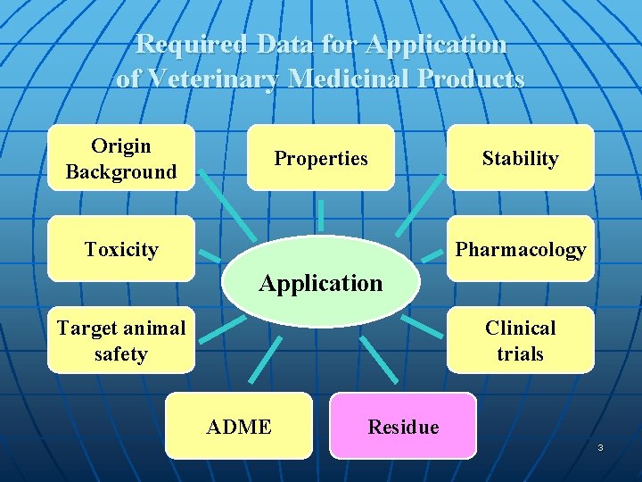
Required Data for Application of Veterinary Medicinal Products Origin Background Properties Toxicity Stability Pharmacology Application Target animal safety Clinical trials ADME Residue 3

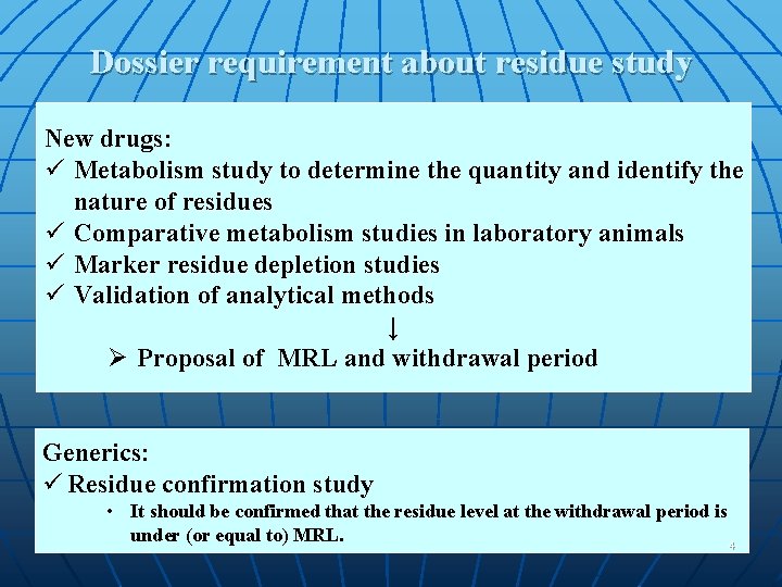
Dossier requirement about residue study New drugs: ü Metabolism study to determine the quantity and identify the nature of residues ü Comparative metabolism studies in laboratory animals ü Marker residue depletion studies ü Validation of analytical methods ↓ Ø Proposal of MRL and withdrawal period Generics: ü Residue confirmation study • It should be confirmed that the residue level at the withdrawal period is under (or equal to) MRL. 4

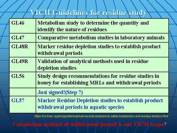
VICH Guidelines for residue study GL 46 GL 47 GL 48 R GL 49 R GL 56 Metabolism study to determine the quantity and identify the nature of residues Comparative metabolism studies in laboratory animals Marker residue depletion studies to establish product withdrawal periods Validation of analytical methods used in residue depletion studies Study design recommendations for residue studies in honey for establishing MRLs and withdrawal periods Just signed!(Step 7) GL 57 Marker Residue Depletion studies to establish product withdrawal periods in aquatic species https: //vichsec. org/en/guidelines/pharmaceuticals/pharma-safety/metabolism-and-residue-kinetics. html Calculation method of withdrawal period is out VICH scope!5

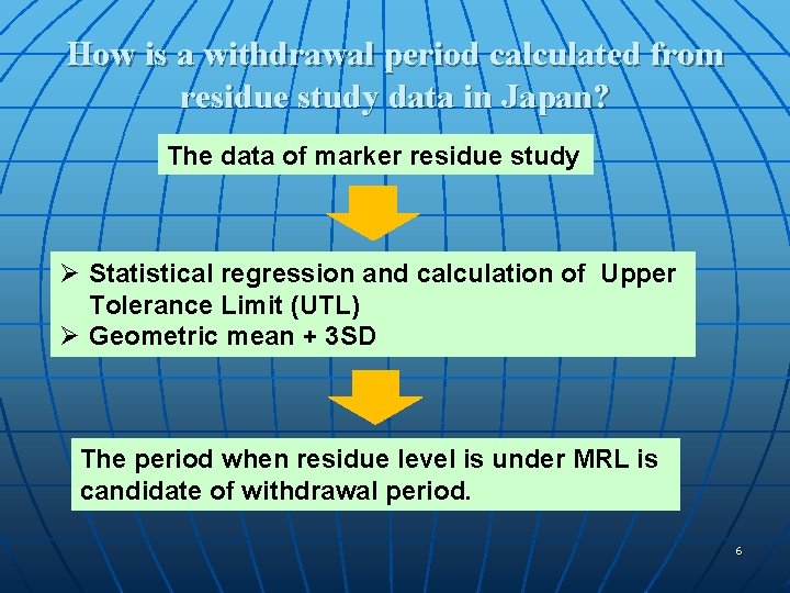
How is a withdrawal period calculated from residue study data in Japan? The data of marker residue study Ø Statistical regression and calculation of Upper Tolerance Limit (UTL) Ø Geometric mean + 3 SD The period when residue level is under MRL is candidate of withdrawal period. 6

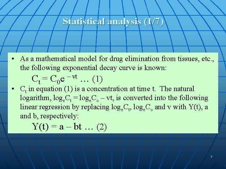
Statistical analysis (1/7) • As a mathematical model for drug elimination from tissues, etc. , the following exponential decay curve is known: Ct = C 0 e – vt … (1) • Ct in equation (1) is a concentration at time t. The natural logarithm, loge. Ct = loge. Co – vt, is converted into the following linear regression by replacing loge. Ct, loge. Co and v with Y(t), a and b, respectively: Y(t) = a – bt … (2) 7

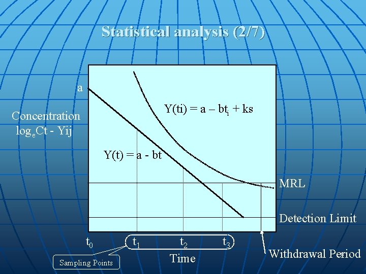
Statistical analysis (2/7) a Y(ti) = a – bti + ks Concentration loge. Ct - Yij Y(t) = a - bt MRL Detection Limit t 0 Sampling Points t 1 t 2 Time t 3 8 Withdrawal Period

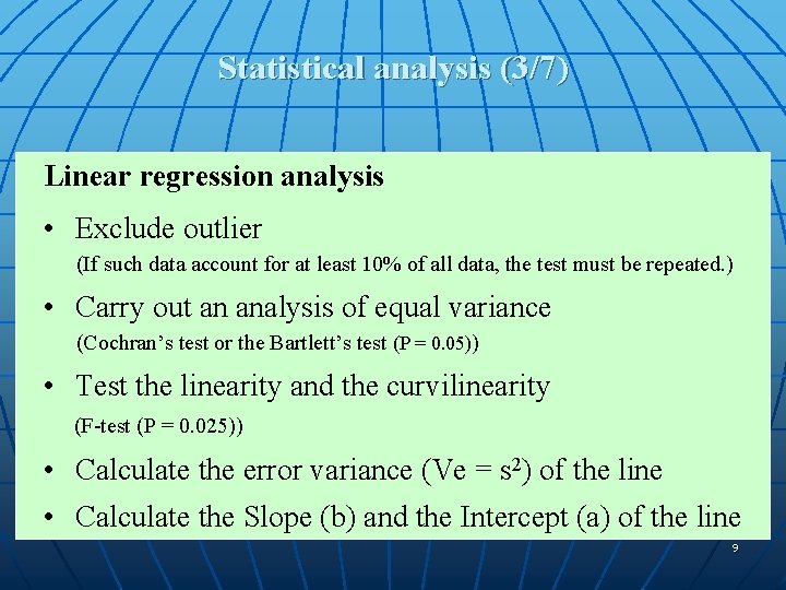
Statistical analysis (3/7) Linear regression analysis • Exclude outlier (If such data account for at least 10% of all data, the test must be repeated. ) • Carry out an analysis of equal variance (Cochran’s test or the Bartlett’s test (P = 0. 05)) • Test the linearity and the curvilinearity (F-test (P = 0. 025)) • Calculate the error variance (Ve = s 2) of the line • Calculate the Slope (b) and the Intercept (a) of the line 9

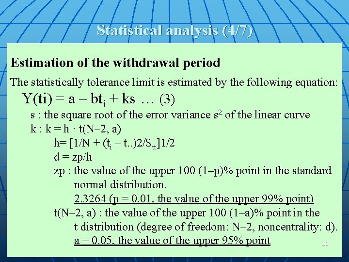
Statistical analysis (4/7) Estimation of the withdrawal period The statistically tolerance limit is estimated by the following equation: Y(ti) = a – bti + ks … (3) s : the square root of the error variance s 2 of the linear curve k : k = h · t(N– 2, a) h= [1/N + (ti – t. . )2/Stt]1/2 d = zp/h zp : the value of the upper 100 (1–p)% point in the standard normal distribution. 2. 3264 (p = 0. 01, the value of the upper 99% point) t(N– 2, a) : the value of the upper 100 (1–a)% point in the t distribution (degree of freedom: N– 2, noncentrality: d). a = 0. 05, the value of the upper 95% point 10

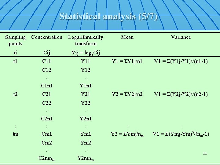
Statistical analysis (5/7) Sampling Concentration points Logarithmically transform Mean Variance Y 1 = ΣY 1 j/n 1 V 1 = Σ(Y 1 j-Y 1)2/(n 1 -1) Y 2 = ΣY 2 j/n 2 V 1 = Σ(Y 2 j-Y 2)2/(n 2 -1) ti Cij Yij = loge. Cij t 1 C 11 Y 11 C 12 Y 12 : : C 1 n 1 Y 1 n 1 C 21 Y 21 C 22 Y 22 : : C 2 n 1 Y 2 n 1 : : : tm Cm 1 Y 2 = ΣYmj/nm V 1 = Σ(Ymj-Ym)2/(nm-1) Cm 2 Ym 2 : : C 2 mnm Y 2 mnm t 2 11

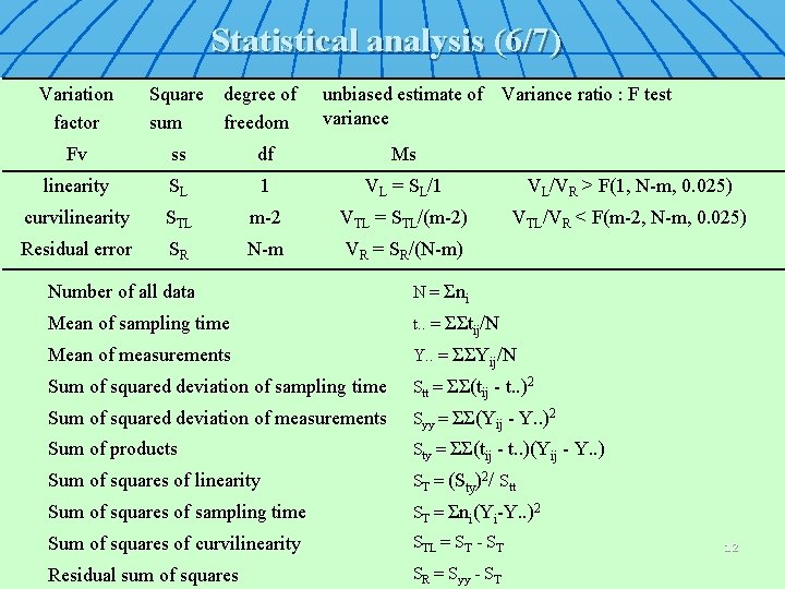
Statistical analysis (6/7) Variation factor Square sum degree of freedom unbiased estimate of Variance ratio : F test variance Fv ss df Ms linearity SL 1 VL = SL/1 VL/VR > F(1, N-m, 0. 025) curvilinearity STL m-2 VTL = STL/(m-2) VTL/VR < F(m-2, N-m, 0. 025) Residual error SR N-m VR = SR/(N-m) Number of all data N = Σni Mean of sampling time t. . = ΣΣtij/N Mean of measurements Y. . = ΣΣYij/N Sum of squared deviation of sampling time Stt = ΣΣ(tij - t. . )2 Sum of squared deviation of measurements Syy = ΣΣ(Yij - Y. . )2 Sum of products Sty = ΣΣ(tij - t. . )(Yij - Y. . ) Sum of squares of linearity ST = (Sty)2/ Stt Sum of squares of sampling time ST = Σni(Yi-Y. . )2 Sum of squares of curvilinearity STL = ST - ST Residual sum of squares SR = Syy - ST 12

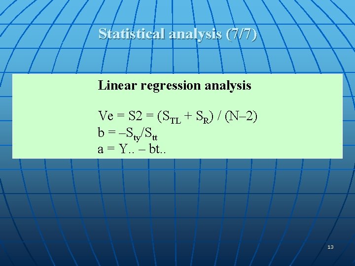
Statistical analysis (7/7) Linear regression analysis Ve = S 2 = (STL + SR) / (N– 2) b = –Sty/Stt a = Y. . – bt. . 13

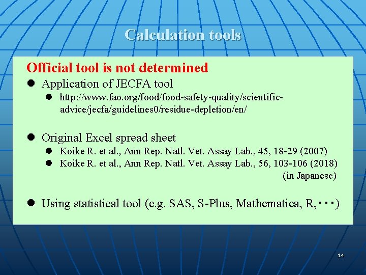
Calculation tools Official tool is not determined l Application of JECFA tool l http: //www. fao. org/food-safety-quality/scientificadvice/jecfa/guidelines 0/residue-depletion/en/ l Original Excel spread sheet l Koike R. et al. , Ann Rep. Natl. Vet. Assay Lab. , 45, 18 -29 (2007) l Koike R. et al. , Ann Rep. Natl. Vet. Assay Lab. , 56, 103 -106 (2018) (in Japanese) l Using statistical tool (e. g. SAS, S-Plus, Mathematica, R, ・・・) 14

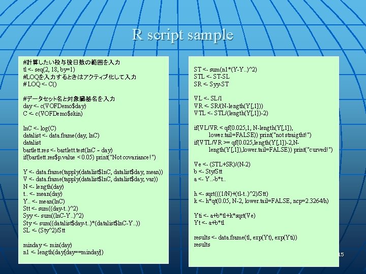
R script sample #計算したい投与後日数の範囲を入力 tl <- seq(2, 18, by=1) #LOQを入力するときはアクティブ化して入力 # LOQ <- C() ST <- sum(n 1*(Y-Y. . )^2) STL <- ST-SL SR <- Syy-ST #データセット名と対象臓器名を入力 day <- c(VOFDemo$day) C <- c(VOFDemo$skin) VL <- SL/1 VR <- SR/(N-length(Y[, 1])) VTL <- STL/(length(Y[, 1])-2) ln. C <- log(C) datalist <- data. frame(day, ln. C) datalist bartlett. res <- bartlett. test(ln. C ~ day) if(bartlett. res$p. value < 0. 05) print("Not covariance!") if(VL/VR < qf(0. 025, 1, N-length(Y[, 1]), lower. tail=FALSE)) print("not straigtht!") if(VTL/VR >= qf(0. 025, length(Y[, 1])-2, Nlength(Y[, 1]), lower. tail=FALSE)) print("curved!") Y <- data. frame(tapply(datalist$ln. C, datalist$day, mean)) V <- data. frame(tapply(datalist$ln. C, datalist$day, var)) N <- length(day) t. . <- mean(day) Y. . <- mean(ln. C) Stt <- sum((day-t. . )^2) Syy <- sum((ln. C-Y. . )^2) Sty <- sum((datalist$day-t. . )*(datalist$ln. C-Y. . )) SL <- (Sty^2)/Stt minday <- min(day) n 1 <- length(day[day==minday]) Ve <- (STL+SR)/(N-2) b <- Sty/Stt a <- Y. . -b*t. . h <- sqrt(((1/N)+(tl-t. . )^2)/Stt) k <- h*qt(0. 05, N-2, lower. tail=FALSE, ncp=2. 3264/h) Yti <- a+b*tl+k*sqrt(Ve) Yt <- a+b*tl results <- data. frame(tl, exp(Yt), exp(Yti)) results 15

Home Page Address Ministry of Agriculture, Forestry and Fisheries http: //www. maff. go. jp/e/index. html National Veterinary Assay Laboratory http: //www. maff. go. jp/nval/english/index. html Food Safety Committee (FSC) http: //www. fsc. go. jp/english/index. html Ministry of Health, Labour and Welfare(MHLW) http: //www. mhlw. go. jp/English/ 16

Thank you! 17