Where and when should one hope to find

Where and when should one hope to find added value from dynamical downscaling of GCM data? René Laprise Director, Centre ESCER (Étude et Simulation du Climat à l’Échelle Régionale) Professor, UQAM (Université du Québec à Montréal) WCRP Regional Climate Workshop: Facilitating the production of climate information and its use in impact and adaptation work Lille (France), 14 -16 June 2010

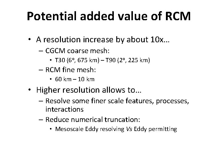
Potential added value of RCM • A resolution increase by about 10 x… – CGCM coarse mesh: • T 30 (6 o, 675 km) – T 90 (2 o, 225 km) – RCM fine mesh: • 60 km – 10 km • Higher resolution allows to… – Resolve some finer scale features, processes, interactions – Reduce numerical truncation: • Mesoscale Eddy resolving Vs Eddy permitting

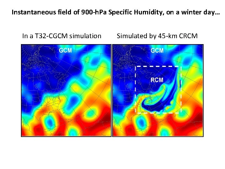
Instantaneous field of 900 -h. Pa Specific Humidity, on a winter day… In a T 32 -CGCM simulation Simulated by 45 -km CRCM

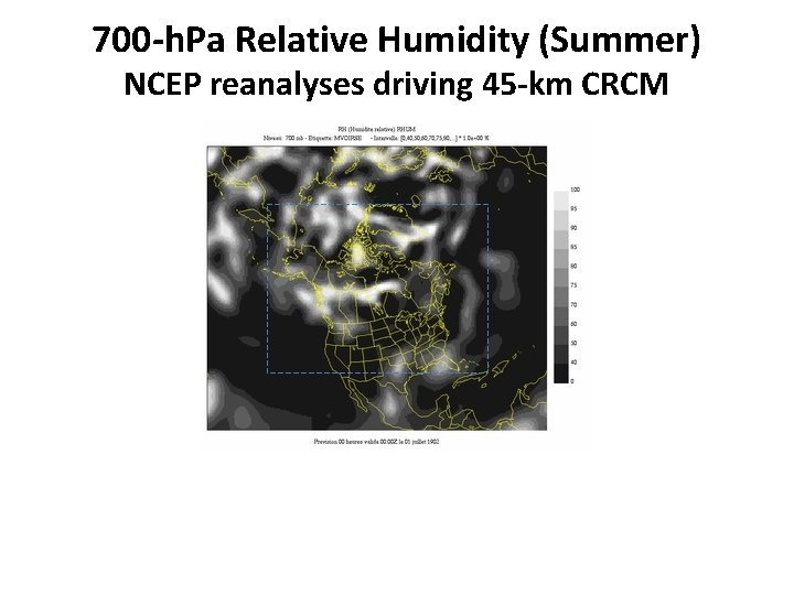
700 -h. Pa Relative Humidity (Summer) NCEP reanalyses driving 45 -km CRCM

– Clear to the naked eye in the time evolution of RCM-simulated fields – But what about climatological (timemean) fields?

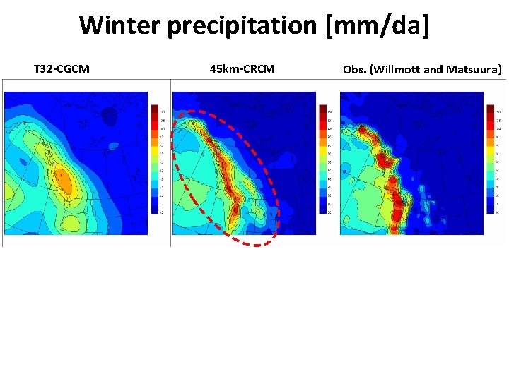
Winter precipitation [mm/da] T 32 -CGCM 45 km-CRCM Obs. (Willmott and Matsuura)

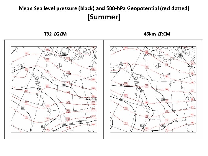
Mean Sea level pressure (black) and 500 -h. Pa Geopotential (red dotted) [Summer] T 32 -CGCM 45 km-CRCM

– Clear to the naked eye in the time evolution of RCM-simulated fields – But what about climatological (time-mean) fields? • Yes for fields strongly affected by local, stationary forcings, such as mountains, land-sea contrast, etc. • Usually not for other fields • But there are exceptions…

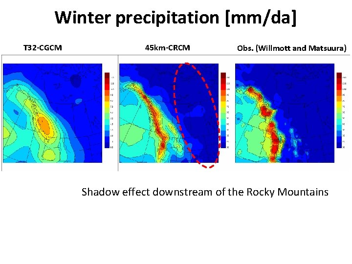
Winter precipitation [mm/da] T 32 -CGCM 45 km-CRCM Obs. (Willmott and Matsuura) Shadow effect downstream of the Rocky Mountains

– Clear to the naked eye in the time evolution of RCMsimulated fields – But what about climatological (time-mean) fields? • Yes for fields strongly affected by local, stationary forcings, such as mountains, land-sea contrast, etc. • Usually not for other fields • But on occasion there are detectable “large-scale” effects resulting from “fine-scale” forcing: A sort of indirect effect of reduced truncation

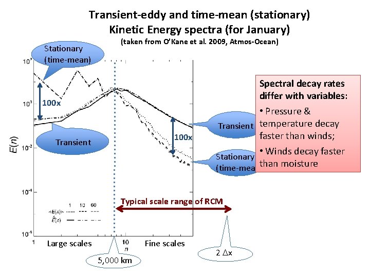
Transient-eddy and time-mean (stationary) Kinetic Energy spectra (for January) Stationary (time-mean) (taken from O’Kane et al. 2009, Atmos-Ocean) 100 x Transient Spectral decay rates differ with variables: • Pressure & Transient temperature decay faster than winds; • Winds decay faster Stationary (time-mean)than moisture Typical scale range of RCM Fine scales Large scales 5, 000 km 2 Dx

– Clear to the naked eye in the time evolution of RCMsimulated fields – But what about climatological (time-mean) fields? • Yes for fields strongly affected by local, stationary forcings, such as mountains, land-sea contrast, etc. • Usually not for other fields: – Time-averaged (stationary-eddy) fields variance mostly contained in large-scale part of the spectrum; well resolved by coarse-mesh GCM – The small-scale part of the spectrum (added by hires RCM) is dominated by transient eddies (not seen in time-mean fields)

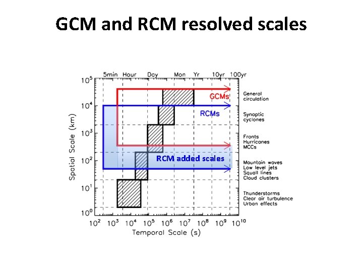
Scale separation • For most atmospheric fields, the variance spectrum of time-averaged (climatological) fields is dominated by large scales: – This hides the potential added value of increased resolution contained in fine scales • Scale separation is a useful (sometimes necessary) tool to identify RCM potential added value

GCM and RCM resolved scales RCM added scales

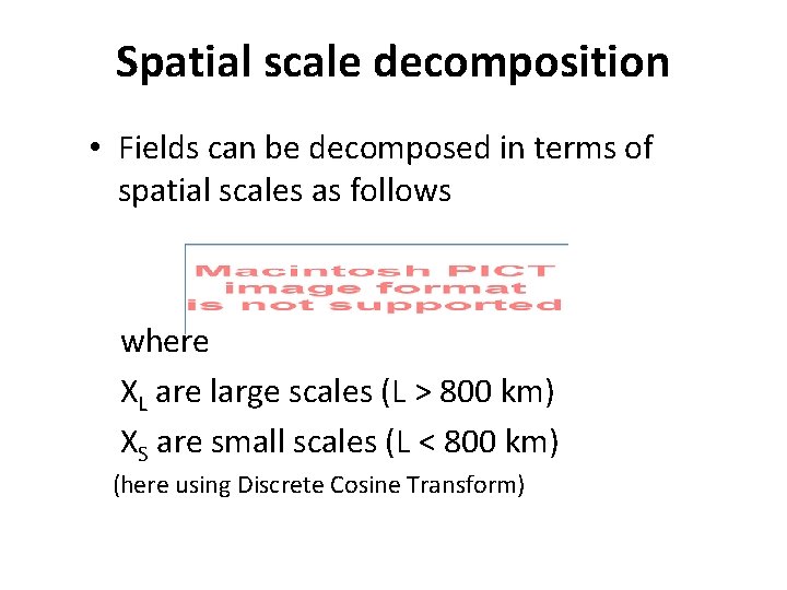
Spatial scale decomposition • Fields can be decomposed in terms of spatial scales as follows where XL are large scales (L > 800 km) XS are small scales (L < 800 km) (here using Discrete Cosine Transform)

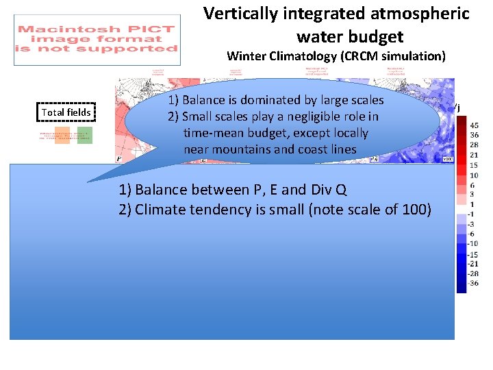
Vertically integrated atmospheric water budget Winter Climatology (CRCM simulation) Total fields Large scales L > 800 km Small scales L < 800 km 1) Balance is dominated by large scales 2) Small scales play a negligible role in time-mean budget, except locally near mountains and coast lines 1) Balance between P, E and Div Q 2) Climate tendency is small (note scale of 100) mm/j

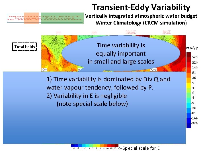
Transient-Eddy Variability Vertically integrated atmospheric water budget Winter Climatology (CRCM simulation) Total fields Large scales L > 800 km Time variability is equally important in small and large scales 1) Time variability is dominated by Div Q and water vapour tendency, followed by P. 2) Variability in E is negligible (note special scale below) Small scales L < 800 km <- Special scale for E mm 2/j 2

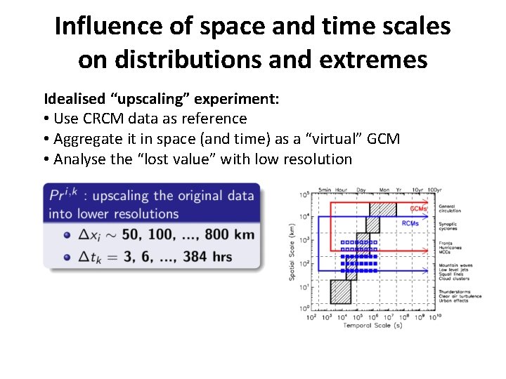
Influence of space and time scales on distributions and extremes Idealised “upscaling” experiment: • Use CRCM data as reference • Aggregate it in space (and time) as a “virtual” GCM • Analyse the “lost value” with low resolution

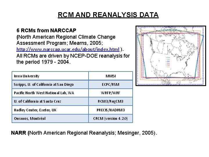
RCM AND REANALYSIS DATA 6 RCMs from NARCCAP (North American Regional Climate Change Assessment Program; Mearns, 2005; http: //www. narccap. ucar. edu/about/index. html ). All RCMs are driven by NCEP-DOE reanalysis for the period 1979 - 2004. Iowa University MM 5 I Scripps, U. of California at San Diego ECPC/RSM Pacific North West National Lab, WA WRFP/WRF U. of California at Santa Cruz Hadley Center, Exeter, UK Ouranos, Montréal RCM 3/Reg. CM 3 PRECIS/HADRM 3 CRCM (version 4. 2. 0) NARR (North American Regional Reanalysis; Mesinger, 2005).

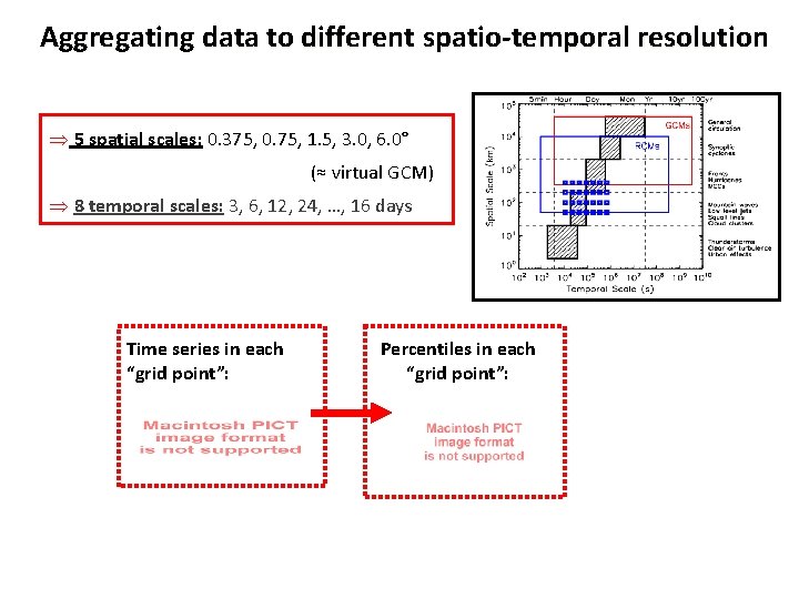
Aggregating data to different spatio-temporal resolution Þ 5 spatial scales: 0. 375, 0. 75, 1. 5, 3. 0, 6. 0° (≈ virtual GCM) Þ 8 temporal scales: 3, 6, 12, 24, …, 16 days Time series in each “grid point”: Percentiles in each “grid point”:

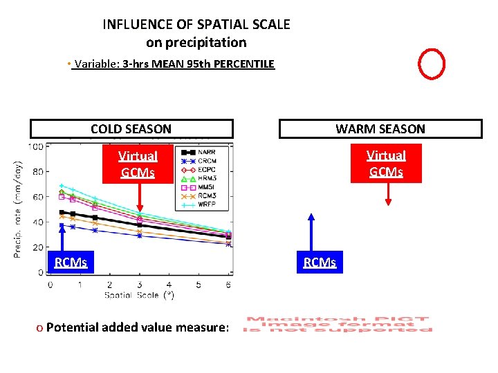
INFLUENCE OF SPATIAL SCALE on precipitation • Variable: 3 -hrs MEAN 95 th PERCENTILE COLD SEASON WARM SEASON Virtual GCMs RCMs o Potential added value measure: RCMs

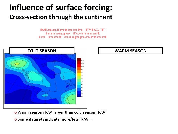
Influence of surface forcing: Cross-section through the continent COLD SEASON o Warm season r. PAV larger than cold season r. PAV o Some datasets indicate more/less r. PAV… WARM SEASON

Conclusions • The main potential added value (PAV) of high-resolution RCM is contained in the fine scales – Although some large-scale effects may be felt as a result of small-scale processes affecting large scales • Do not look for PAV in time-averaged, climatological quantities: – Except where there is strong local stationary forcing (e. g. mountains, land-sea contrast), time averaging tends to remove small scales – Scale separation is a useful, sometimes necessary, tool to identify PAV • Look for PAV in variability statistics: – Transient-eddy variability – Extremes in distributions References: • Laprise, R. de Elía, D. Caya, S. Biner, Ph. Lucas-Picher, E. P. Diaconescu, M. Leduc, A. Alexandru and L. Separovic, 2008: Challenging some tenets of Regional Climate Modelling. Meteor. Atmos. Phys. 100 • Bresson, R. , and R. Laprise, 2009: Scale-decomposed atmospheric water budget over North America as simulated by the Canadian Regional Climate Model for current and future climates. Clim. Dyn. 1 -20 • Di Luca, A. , R. de Elía and R. Laprise: Assessment of the potential added value in multi-RCM simulated precipitation (in preparation)