University of Warwick Department of Sociology 201415 SO

University of Warwick, Department of Sociology, 2014/15 SO 201: SSAASS (Surveys and Statistics) (Richard Lampard) Clustering and Scaling (Week 19)

Distances. . . • Some quantitative techniques derive and/or use distances between variables, or distances between categories within variables, as the basis for the construction of maps or the division of items into sets of similar items. • These include multidimensional scaling, correspondence analysis, and cluster analysis.

Multidimensional scaling (MDS) • MDS is applied to a set of distances between all pairs of categories within a set of categories. • See Coxon (1982); Kruskal and Wish (1978)

Cluster analysis • In cluster analysis, distances between items (cases and/variables) are generated from the raw data, and then used to generate a categorisation of the items. • See Everitt (1993; see also later editions)

Classifying women’s occupations • Dale et al. (1985: see handout) used cluster analysis to develop an ‘alternative’ set of categories for women’s occupations.

The Cambridge Scale • The Cambridge Social Stratification scale was originally derived via the application of multidimensional scaling to occupation-based cross-tabulations matching the occupations of individuals and their ‘associates’. • It subsequently moved in the direction of using correspondence analysis (Prandy 1990; Prandy and Bottero 1998: 2. 6 - see handout).

‘Marriage and the Social Order’ • Prandy and Bottero (1998: handout) applied correspondence analysis to occupation-based cross-tabulations to locate occupations on a number of (highly correlated) occupational scales.

Correspondence analysis • Correspondence analysis in effect partitions the relationship in a cross-tabulation (and more specifically the chi-square statistic) into components reflecting a number of underlying dimensions (see Greenacre 2007). • More specifically, the difference between the distributions of values for two categories is split into components reflecting different underlying dimensions.

Association models • More recently the Cambridge scale and international equivalents have tended to use ‘association models’, which are a form of statistical model that echoes aspects of correspondence analysis. • See Goodman, L. A. 1986. ‘Some useful extensions to the usual correspondence analysis approach and the usual loglinear approach in the analysis of contingency tables (with comments)’, . Int. Statist. Rev. 54: 243 -309. • See also: http: //www. camsis. stir. ac. uk/

Evaluating the NS-SEC • In Rose and Pevalin (2003), various chapters (by Mills and Evans [see extract in handout], Coxon and Fisher, and Fisher) involved the application of cluster analysis, multidimensional scaling, and association models to the relationship between employment relations measures and occupational categories.

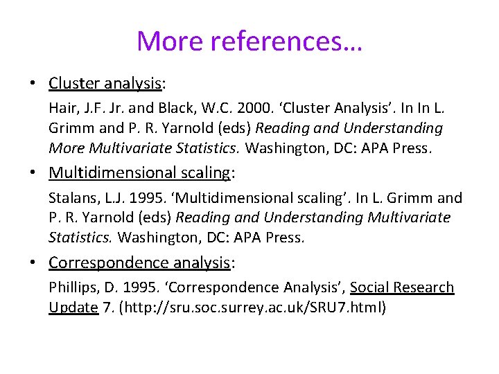
More references… • Cluster analysis: Hair, J. F. Jr. and Black, W. C. 2000. ‘Cluster Analysis’. In In L. Grimm and P. R. Yarnold (eds) Reading and Understanding More Multivariate Statistics. Washington, DC: APA Press. • Multidimensional scaling: Stalans, L. J. 1995. ‘Multidimensional scaling’. In L. Grimm and P. R. Yarnold (eds) Reading and Understanding Multivariate Statistics. Washington, DC: APA Press. • Correspondence analysis: Phillips, D. 1995. ‘Correspondence Analysis’, Social Research Update 7. (http: //sru. soc. surrey. ac. uk/SRU 7. html)

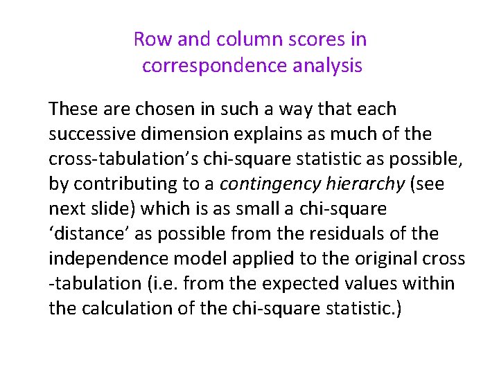
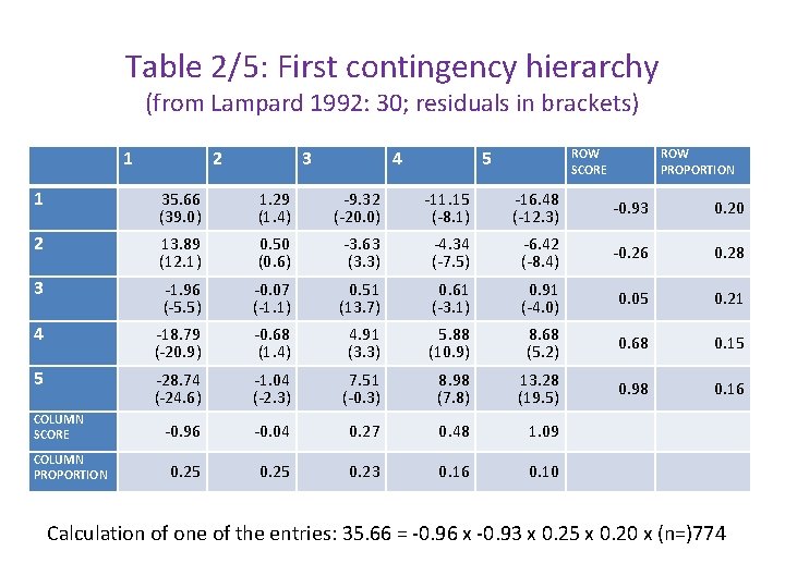
Row and column scores in correspondence analysis These are chosen in such a way that each successive dimension explains as much of the cross-tabulation’s chi-square statistic as possible, by contributing to a contingency hierarchy (see next slide) which is as small a chi-square ‘distance’ as possible from the residuals of the independence model applied to the original cross -tabulation (i. e. from the expected values within the calculation of the chi-square statistic. )

Table 2/5: First contingency hierarchy (from Lampard 1992: 30; residuals in brackets) 1 2 3 4 5 ROW SCORE ROW PROPORTION 1 35. 66 (39. 0) 1. 29 (1. 4) -9. 32 (-20. 0) -11. 15 (-8. 1) -16. 48 (-12. 3) -0. 93 0. 20 2 13. 89 (12. 1) 0. 50 (0. 6) -3. 63 (3. 3) -4. 34 (-7. 5) -6. 42 (-8. 4) -0. 26 0. 28 3 -1. 96 (-5. 5) -0. 07 (-1. 1) 0. 51 (13. 7) 0. 61 (-3. 1) 0. 91 (-4. 0) 0. 05 0. 21 4 -18. 79 (-20. 9) -0. 68 (1. 4) 4. 91 (3. 3) 5. 88 (10. 9) 8. 68 (5. 2) 0. 68 0. 15 5 -28. 74 (-24. 6) -1. 04 (-2. 3) 7. 51 (-0. 3) 8. 98 (7. 8) 13. 28 (19. 5) 0. 98 0. 16 -0. 96 -0. 04 0. 27 0. 48 1. 09 0. 25 0. 23 0. 16 0. 10 COLUMN SCORE COLUMN PROPORTION Calculation of one of the entries: 35. 66 = -0. 96 x -0. 93 x 0. 25 x 0. 20 x (n=)774

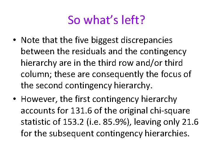
So what’s left? • Note that the five biggest discrepancies between the residuals and the contingency hierarchy are in the third row and/or third column; these are consequently the focus of the second contingency hierarchy. • However, the first contingency hierarchy accounts for 131. 6 of the original chi-square statistic of 153. 2 (i. e. 85. 9%), leaving only 21. 6 for the subsequent contingency hierarchies.