Tomographic algorithm for multiconjugate adaptive optics systems Donald

Tomographic algorithm for multiconjugate adaptive optics systems Donald Gavel Center for Adaptive Optics UC Santa Cruz UCO Lick Observatory NSF Center for Adaptive Optics Laboratory for Adaptive Optics IPAM Workshop on Estimation and Control Problems in

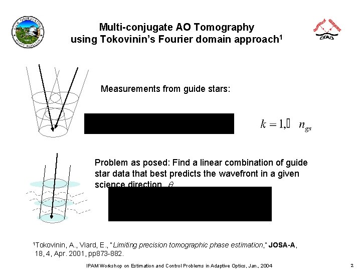
Multi-conjugate AO Tomography using Tokovinin’s Fourier domain approach 1 Measurements from guide stars: Problem as posed: Find a linear combination of guide star data that best predicts the wavefront in a given science direction, q 1 Tokovinin, A. , Viard, E. , “Limiting precision tomographic phase estimation, ” JOSA-A, 18, 4, Apr. 2001, pp 873 -882. IPAM Workshop on Estimation and Control Problems in Adaptive Optics, Jan. , 2004 2

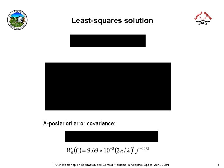
Least-squares solution A-posteriori error covariance: IPAM Workshop on Estimation and Control Problems in Adaptive Optics, Jan. , 2004 3

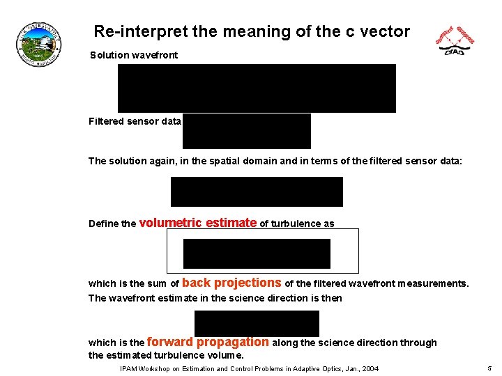
Re-interpret the meaning of the c vector Solution wavefront Filtered sensor data vector: The solution again, in the spatial domain and in terms of the filtered sensor data: Define the volumetric estimate of turbulence as which is the sum of back projections of the filtered wavefront measurements. The wavefront estimate in the science direction is then which is the forward propagation along the science direction through the estimated turbulence volume. IPAM Workshop on Estimation and Control Problems in Adaptive Optics, Jan. , 2004 5

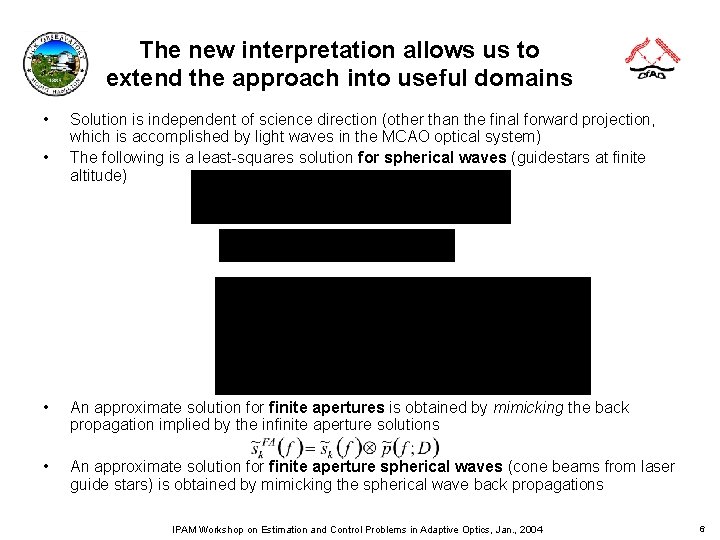
The new interpretation allows us to extend the approach into useful domains • • Solution is independent of science direction (other than the final forward projection, which is accomplished by light waves in the MCAO optical system) The following is a least-squares solution for spherical waves (guidestars at finite altitude) • An approximate solution for finite apertures is obtained by mimicking the back propagation implied by the infinite aperture solutions • An approximate solution for finite aperture spherical waves (cone beams from laser guide stars) is obtained by mimicking the spherical wave back propagations IPAM Workshop on Estimation and Control Problems in Adaptive Optics, Jan. , 2004 6

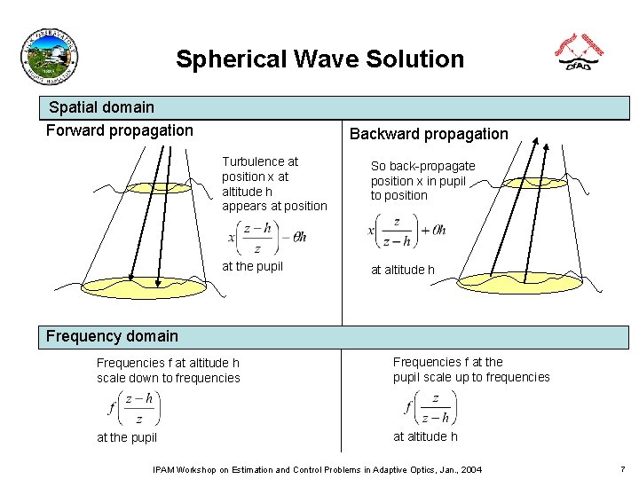
Spherical Wave Solution Spatial domain Forward propagation Backward propagation Turbulence at position x at altitude h appears at position So back-propagate position x in pupil to position at the pupil at altitude h Frequency domain Frequencies f at altitude h scale down to frequencies Frequencies f at the pupil scale up to frequencies at the pupil at altitude h IPAM Workshop on Estimation and Control Problems in Adaptive Optics, Jan. , 2004 7

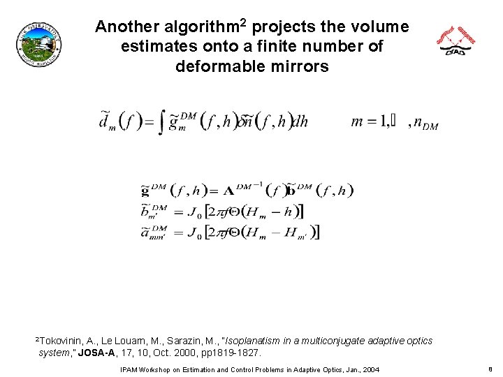
Another algorithm 2 projects the volume estimates onto a finite number of deformable mirrors 2 Tokovinin, A. , Le Louarn, M. , Sarazin, M. , “Isoplanatism in a multiconjugate adaptive optics system, ” JOSA-A, 17, 10, Oct. 2000, pp 1819 -1827. IPAM Workshop on Estimation and Control Problems in Adaptive Optics, Jan. , 2004 8

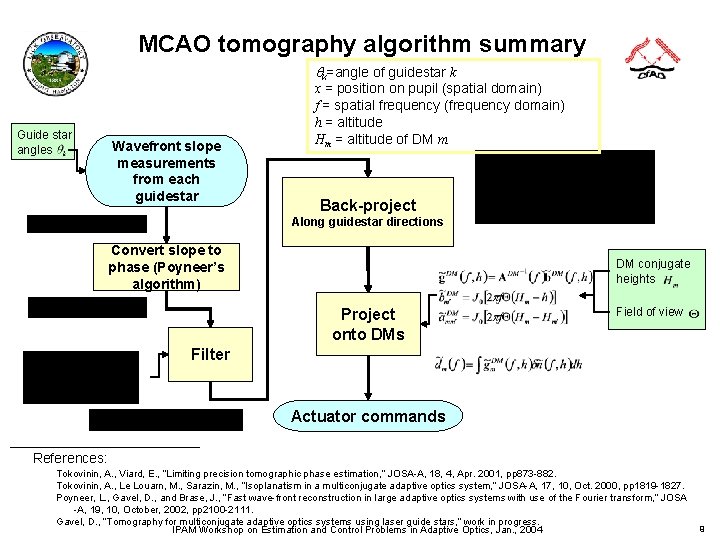
MCAO tomography algorithm summary qk=angle of guidestar k Guide star angles Wavefront slope measurements from each guidestar x = position on pupil (spatial domain) f = spatial frequency (frequency domain) h = altitude Hm = altitude of DM m Back-project Along guidestar directions Convert slope to phase (Poyneer’s algorithm) DM conjugate heights Project onto DMs Field of view Filter Actuator commands References: Tokovinin, A. , Viard, E. , “Limiting precision tomographic phase estimation, ” JOSA-A, 18, 4, Apr. 2001, pp 873 -882. Tokovinin, A. , Le Louarn, M. , Sarazin, M. , “Isoplanatism in a multiconjugate adaptive optics system, ” JOSA-A, 17, 10, Oct. 2000, pp 1819 -1827. Poyneer, L. , Gavel, D. , and Brase, J. , “Fast wave-front reconstruction in large adaptive optics systems with use of the Fourier transform, ” JOSA -A, 19, 10, October, 2002, pp 2100 -2111. Gavel, D. , “Tomography for multiconjugate adaptive optics systems using laser guide stars, ” work in progress. IPAM Workshop on Estimation and Control Problems in Adaptive Optics, Jan. , 2004 9

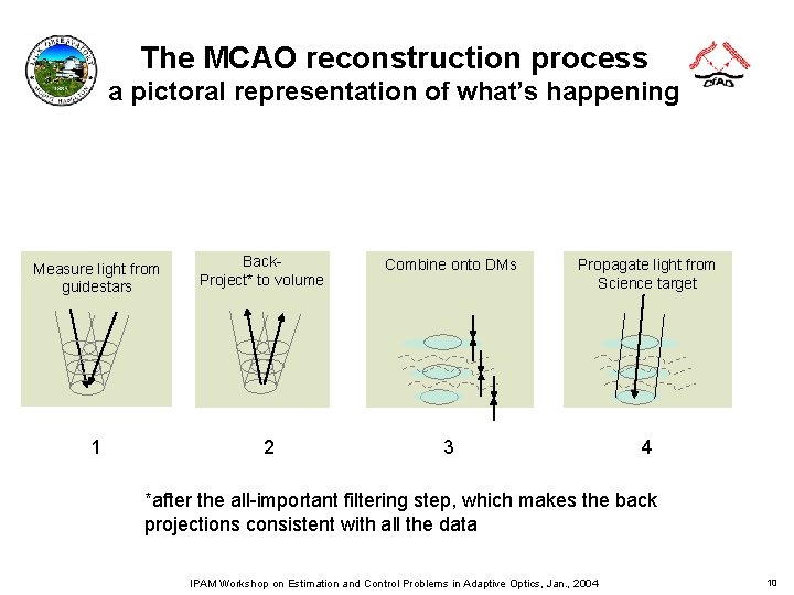
The MCAO reconstruction process a pictoral representation of what’s happening Measure light from guidestars 1 Back. Project* to volume 2 Combine onto DMs Propagate light from Science target 3 4 *after the all-important filtering step, which makes the back projections consistent with all the data IPAM Workshop on Estimation and Control Problems in Adaptive Optics, Jan. , 2004 10

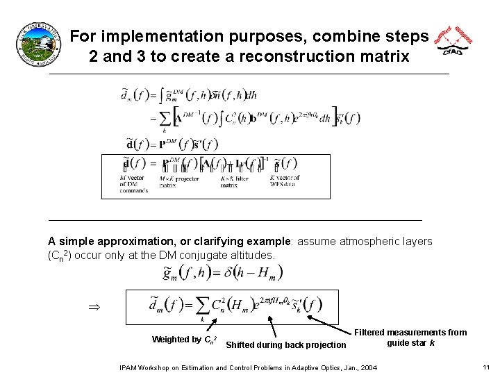
For implementation purposes, combine steps 2 and 3 to create a reconstruction matrix A simple approximation, or clarifying example: assume atmospheric layers (Cn 2) occur only at the DM conjugate altitudes. Þ Weighted by Cn 2 Filtered measurements from guide star k Shifted during back projection IPAM Workshop on Estimation and Control Problems in Adaptive Optics, Jan. , 2004 11

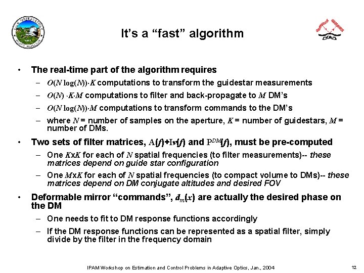
It’s a “fast” algorithm • The real-time part of the algorithm requires – O(N log(N))×K computations to transform the guidestar measurements – O(N) ×K×M computations to filter and back-propagate to M DM’s – O(N log(N))×M computations to transform commands to the DM’s – where N = number of samples on the aperture, K = number of guidestars, M = number of DMs. • Two sets of filter matrices, A(f)+Iv(f) and PDM(f), must be pre-computed – One Kx. K for each of N spatial frequencies (to filter measurements)-- these matrices depend on guide star configuration – One Mx. K for each of N spatial frequencies (to compact volume to DMs)-- these matrices depend on DM conjugate altitudes and desired FOV • Deformable mirror “commands”, dm(x) are actually the desired phase on the DM – One needs to fit to DM response functions accordingly – If the DM response functions can be represented as a spatial filter, simply divide by the filter in the frequency domain IPAM Workshop on Estimation and Control Problems in Adaptive Optics, Jan. , 2004 12

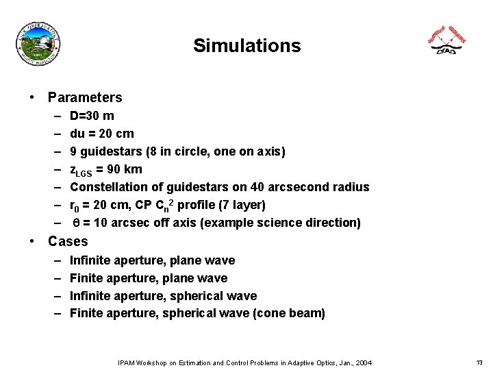
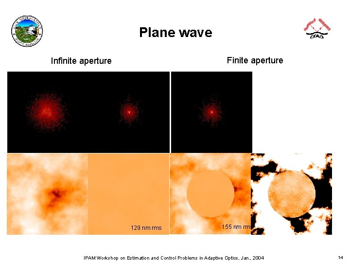
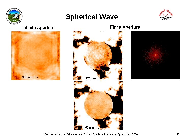
Simulations • Parameters – – – – D=30 m du = 20 cm 9 guidestars (8 in circle, one on axis) z. LGS = 90 km Constellation of guidestars on 40 arcsecond radius r 0 = 20 cm, CP Cn 2 profile (7 layer) q = 10 arcsec off axis (example science direction) • Cases – – Infinite aperture, plane wave Finite aperture, plane wave Infinite aperture, spherical wave Finite aperture, spherical wave (cone beam) IPAM Workshop on Estimation and Control Problems in Adaptive Optics, Jan. , 2004 13

Plane wave Finite aperture Infinite aperture 129 nm rms 155 nm rms IPAM Workshop on Estimation and Control Problems in Adaptive Optics, Jan. , 2004 14

Spherical Wave Finite Aperture Infinite Aperture 388 nm rms 421 nm rms 155 nm rms IPAM Workshop on Estimation and Control Problems in Adaptive Optics, Jan. , 2004 15

Movie IPAM Workshop on Estimation and Control Problems in Adaptive Optics, Jan. , 2004 16

Conclusions • MCAO Fourier domain tomography analyses can be extended to spherical waves and finite apertures, and suggest practical real-time reconstructors • Finite aperture algorithms “mimic” their infinite aperture equivalents • Fourier domain reconstructors are fast – Useful for fast exploration of parameter space – Could be good pre-conditioners for iterative methods – if they aren’t sufficiently accurate on their own • Difficulties – Sampling 30 m aperture finely enough (on my PC) – Numerical singularity of filter matrices at some spatial frequencies – Spherical wave tomographic error appears to be high in simulations, but this may be due to the numerics of rescaling/resampling (we’re working on this) – Not clear how to extend the infinite aperture spherical wave solution to frequency domain covariance analysis (it mixes and thus cross-correlates different frequencies) IPAM Workshop on Estimation and Control Problems in Adaptive Optics, Jan. , 2004 17