Analysis and Design of an Adaptive Virtual Queue

Analysis and Design of an Adaptive Virtual Queue (AVQ) Algorithm for Active Queue Managment Srisankar Kunniyur and R. Srikant SIGCOMM’ 01 San Diego ACN: AVQ 1

AVQ Outline • • • AVQ concepts, notation and algorithm Fluid-flow model and Theorem 1 Simulations Stability Analysis of AVQ Conclusions ACN: AVQ 2

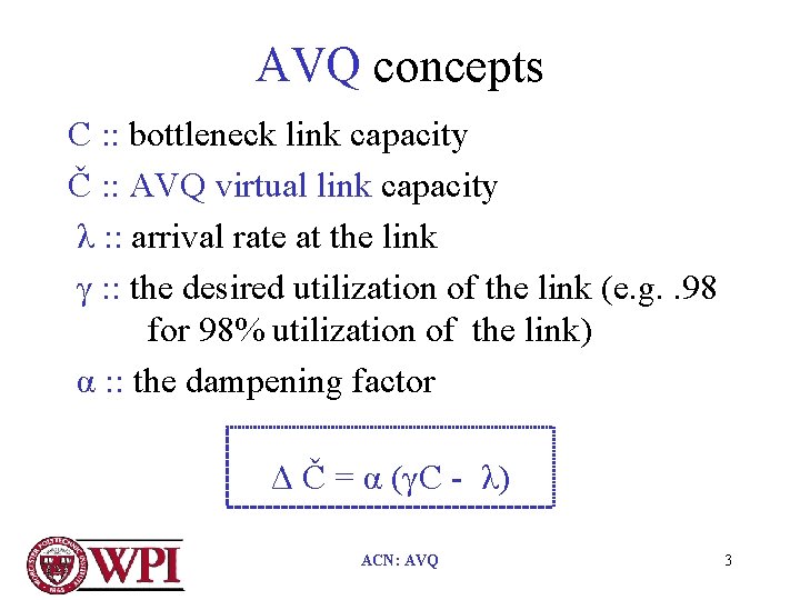
AVQ concepts C : : bottleneck link capacity Č : : AVQ virtual link capacity λ : : arrival rate at the link γ : : the desired utilization of the link (e. g. . 98 for 98% utilization of the link) α : : the dampening factor Δ Č = α (γC - λ) ACN: AVQ 3

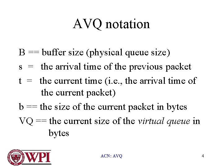
AVQ notation B == buffer size (physical queue size) s = the arrival time of the previous packet t = the current time (i. e. , the arrival time of the current packet) b == the size of the current packet in bytes VQ == the current size of the virtual queue in bytes ACN: AVQ 4

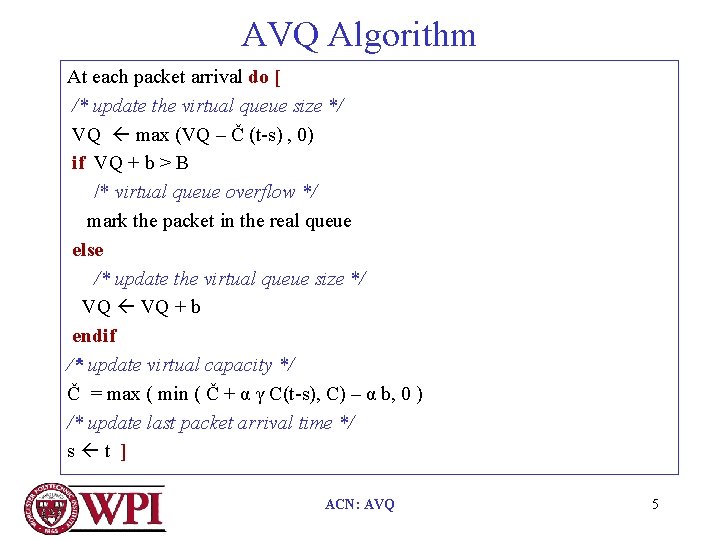
AVQ Algorithm At each packet arrival do [ /* update the virtual queue size */ VQ max (VQ – Č (t-s) , 0) if VQ + b > B /* virtual queue overflow */ mark the packet in the real queue else /* update the virtual queue size */ VQ + b endif /* update virtual capacity */ Č = max ( min ( Č + α γ C(t-s), C) – α b, 0 ) /* update last packet arrival time */ s t ] ACN: AVQ 5

Fluid-flow Model of TCP • Assume N TCP flows with common roundtrip propagation delay d. • Neglect slow-start and the time-out behavior. • Use the utility function – 1/d 2 x • xi is a variable corresponding to the flow rate of the ith flow. • xi = Wi / d gets us back to window control algorithm. ACN: AVQ 6

Significance of Theorem 1 • α determines indirectly how quickly to adapt the marking probability at the link to changing conditions • How do we choose α ? • Given estimates for d, N, and γ, Theorem 1 defines a bounds on α (α < α*) such that the modeled system is stable! ACN: AVQ 7

Let’s pause to think • These authors attempt to validate their model via a series of simulations. • Why? • To convince you that ‘unrealistic’ assumptions do not hurt the applicability of their model. {This is a standard technique!!} ACN: AVQ 8

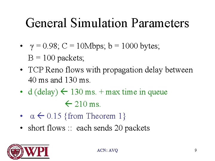
General Simulation Parameters • γ = 0. 98; C = 10 Mbps; b = 1000 bytes; B = 100 packets; • TCP Reno flows with propagation delay between 40 ms and 130 ms. • d (delay) 130 ms. + max time in queue 210 ms. • α 0. 15 {from Theorem 1} • short flows : : each sends 20 packets ACN: AVQ 9

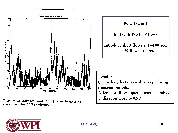
Experiment 1 Start with 180 FTP flows. Introduce short flows at t =100 sec. at 30 flows per sec. Results: Queue length stays small except during transient periods. After short flows, queue length stabilizes. Utilization close to 0. 98 ACN: AVQ 10

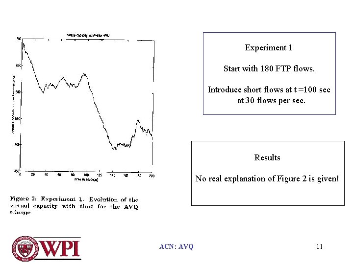
Experiment 1 Start with 180 FTP flows. Introduce short flows at t =100 sec at 30 flows per sec. Results No real explanation of Figure 2 is given! ACN: AVQ 11

Other AQM Algorithms • • RED Random Early Marking (REM) PI Controller Gibbens- Kelly Virtual Queue (GKVQ) ACN: AVQ 12

Random Early Marking (REM) • REM varies mark probability in a manner such that the goal is to keep the queue length near qref. • The probability is updated every T sec. • REM is sensitive to φ ACN: AVQ 13

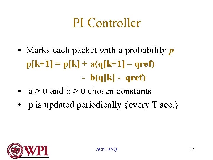
PI Controller • Marks each packet with a probability p p[k+1] = p[k] + a(q[k+1] – qref) - b(q[k] - qref) • a > 0 and b > 0 chosen constants • p is updated periodically {every T sec. } ACN: AVQ 14

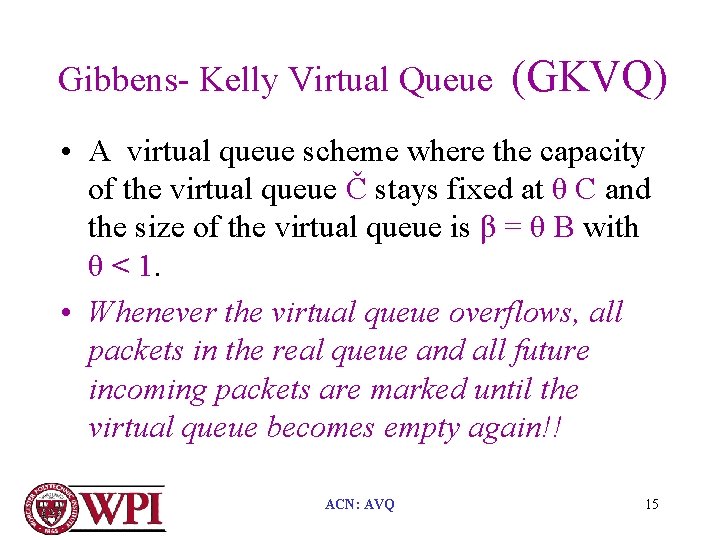
Gibbens- Kelly Virtual Queue (GKVQ) • A virtual queue scheme where the capacity of the virtual queue Č stays fixed at θ C and the size of the virtual queue is β = θ B with θ < 1. • Whenever the virtual queue overflows, all packets in the real queue and all future incoming packets are marked until the virtual queue becomes empty again!! ACN: AVQ 15

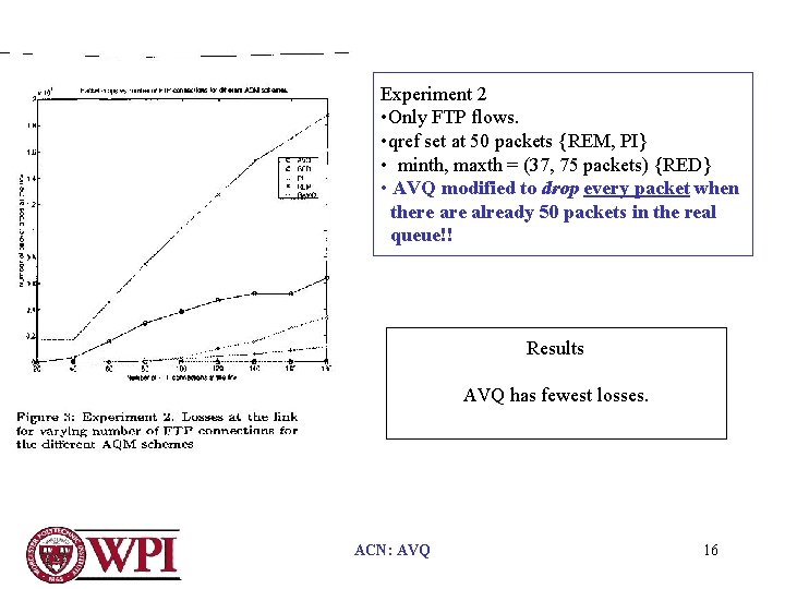
Experiment 2 • Only FTP flows. • qref set at 50 packets {REM, PI} • minth, maxth = (37, 75 packets) {RED} • AVQ modified to drop every packet when there already 50 packets in the real queue!! Results AVQ has fewest losses. ACN: AVQ 16

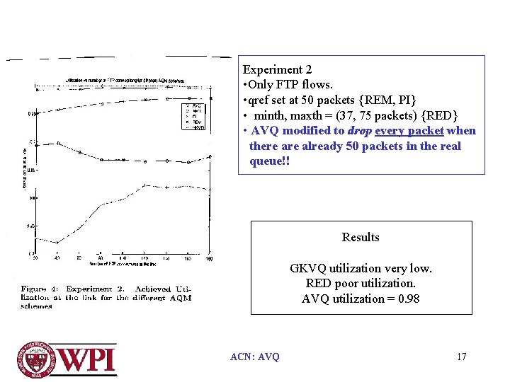
Experiment 2 • Only FTP flows. • qref set at 50 packets {REM, PI} • minth, maxth = (37, 75 packets) {RED} • AVQ modified to drop every packet when there already 50 packets in the real queue!! Results GKVQ utilization very low. RED poor utilization. AVQ utilization = 0. 98 ACN: AVQ 17

Experiment 2 • number of flows changed by increasing number of flows over interval • qref set at 50 packets {REM, PI} • minth, maxth = (37, 75 packets) {RED} • AVQ modified to drop every packet when there already 50 packets in the real queue!! Results RED near 40 PI worse with more flows REM does not make sense? ACN: AVQ 18

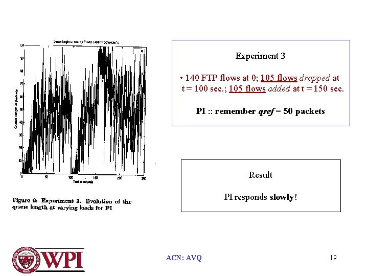
Experiment 3 • 140 FTP flows at 0; 105 flows dropped at t = 100 sec. ; 105 flows added at t = 150 sec. PI : : remember qref = 50 packets Result PI responds slowly! ACN: AVQ 19

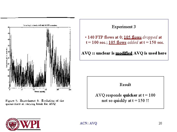
Experiment 3 • 140 FTP flows at 0; 105 flows dropped at t = 100 sec. ; 105 flows added at t = 150 sec. AVQ : : unclear is modified AVQ is used here Result AVQ responds quicker at t = 100 not so quickly at t = 150 !! ACN: AVQ 20

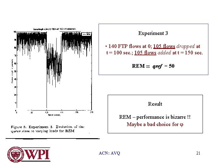
Experiment 3 • 140 FTP flows at 0; 105 flows dropped at t = 100 sec. ; 105 flows added at t = 150 sec. REM : : qref = 50 Result REM – performance is bizarre !! Maybe a bad choice for φ ACN: AVQ 21

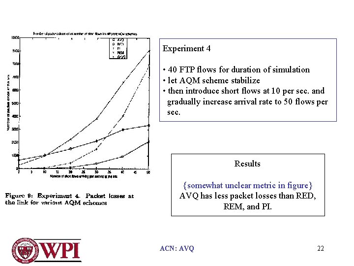
Experiment 4 • 40 FTP flows for duration of simulation • let AQM scheme stabilize • then introduce short flows at 10 per sec. and gradually increase arrival rate to 50 flows per sec. Results {somewhat unclear metric in figure} AVQ has less packet losses than RED, REM, and PI. ACN: AVQ 22

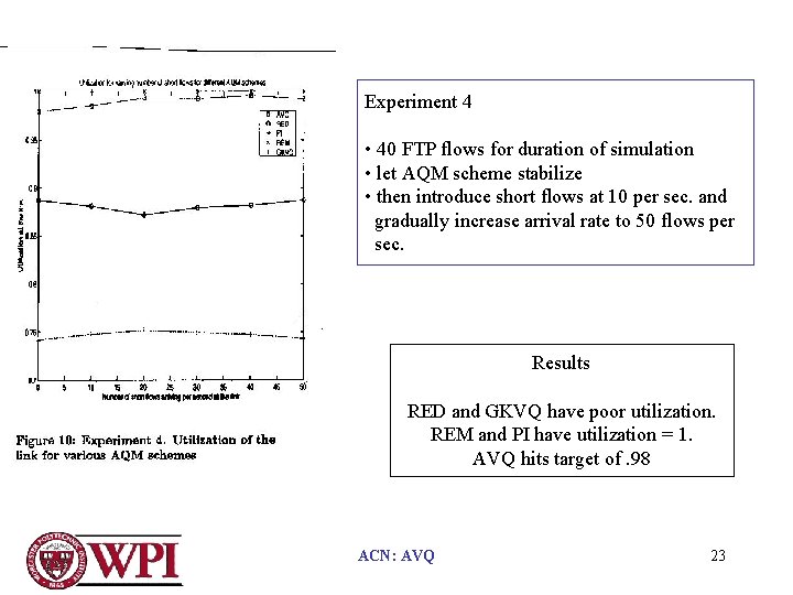
Experiment 4 • 40 FTP flows for duration of simulation • let AQM scheme stabilize • then introduce short flows at 10 per sec. and gradually increase arrival rate to 50 flows per sec. Results RED and GKVQ have poor utilization. REM and PI have utilization = 1. AVQ hits target of. 98 ACN: AVQ 23

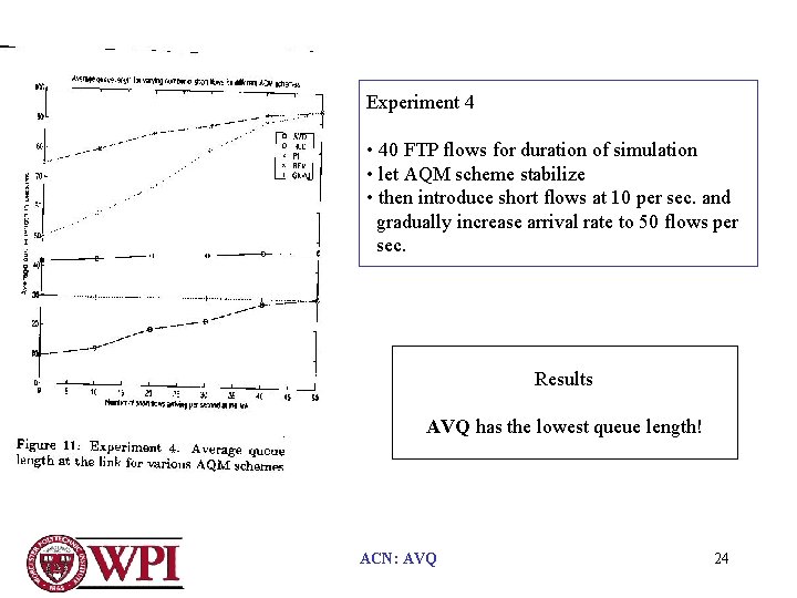
Experiment 4 • 40 FTP flows for duration of simulation • let AQM scheme stabilize • then introduce short flows at 10 per sec. and gradually increase arrival rate to 50 flows per sec. Results AVQ has the lowest queue length! ACN: AVQ 24

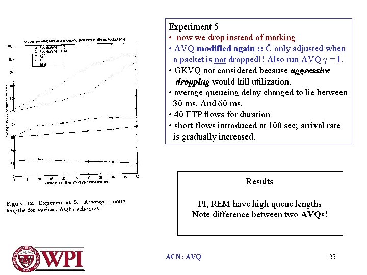
Experiment 5 • now we drop instead of marking • AVQ modified again : : Č only adjusted when a packet is not dropped!! Also run AVQ γ = 1. • GKVQ not considered because aggressive dropping would kill utilization. • average queueing delay changed to lie between 30 ms. And 60 ms. • 40 FTP flows for duration • short flows introduced at 100 sec; arrival rate is gradually increased. Results PI, REM have high queue lengths Note difference between two AVQs! ACN: AVQ 25

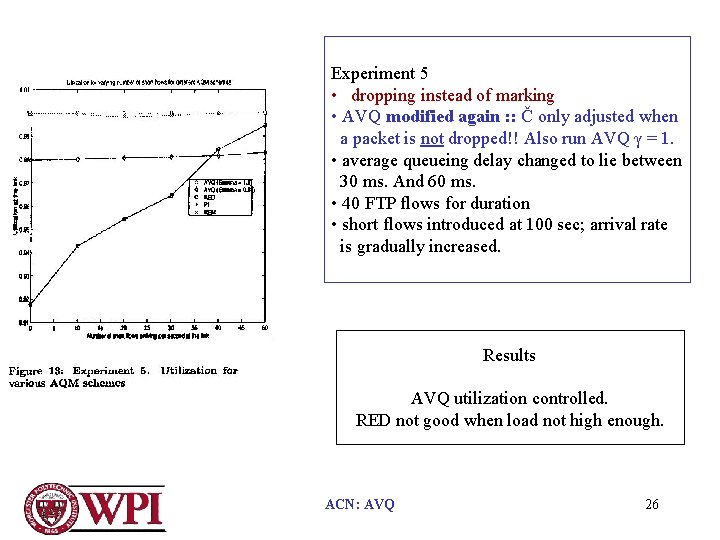
Experiment 5 • dropping instead of marking • AVQ modified again : : Č only adjusted when a packet is not dropped!! Also run AVQ γ = 1. • average queueing delay changed to lie between 30 ms. And 60 ms. • 40 FTP flows for duration • short flows introduced at 100 sec; arrival rate is gradually increased. Results AVQ utilization controlled. RED not good when load not high enough. ACN: AVQ 26

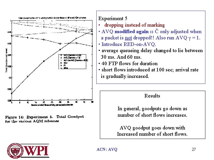
Experiment 5 • dropping instead of marking • AVQ modified again : : Č only adjusted when a packet is not dropped!! Also run AVQ γ = 1. • Introduce RED-on-AVQ. • average queueing delay changed to lie between 30 ms. And 60 ms. • 40 FTP flows for duration • short flows introduced at 100 sec; arrival rate is gradually increased. Results In general, goodputs go down as number of short flows increases. AVQ goodput goes down with Increased number of short flows. ACN: AVQ 27

Stability Analysis of AVQ • To authors Theorem 1 is the main result of the paper. • Math assumes a fixed d. • For stability N must be above a minimum. • Five other theorems discussed. ACN: AVQ 28

Conclusions • Paper used fluid-flow model and assumptions to derive theorem 1. • The AVQ algorithm is based on update equation at link. • Simulations are somewhat contrived and the AVQ algorithm is modified twice to fit specific simulations. {simulation efforts are sloppy} • Authors claim AVQ provides high utilization with low delay, but modified AVQ seems like a kludge. ACN: AVQ 29