TFAWS Interdisciplinary Paper Session ReducedOrder Modeling for Rapid

TFAWS Interdisciplinary Paper Session Reduced-Order Modeling for Rapid Thermal Analysis and Evaluation of Spacecraft Derek Hengeveld Senior Engineer | Load. Path dhengeveld@loadpath. com Thermal & Fluids Analysis Workshop TFAWS 2016 August 1 -5, 2016 NASA Ames Research Center Mountain View, CA

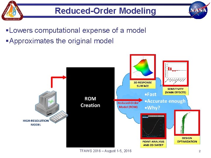
Reduced-Order Modeling §Lowers computational expense of a model §Approximates the original model TFAWS 2016 – August 1 -5, 2016 2

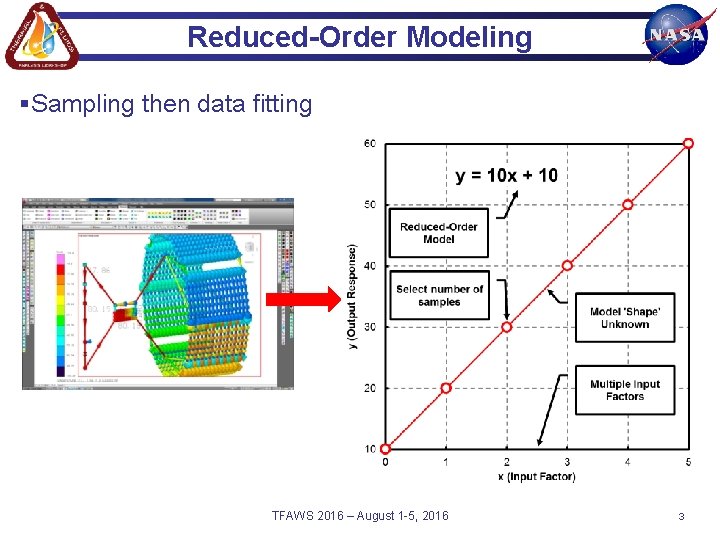
Reduced-Order Modeling §Sampling then data fitting TFAWS 2016 – August 1 -5, 2016 3

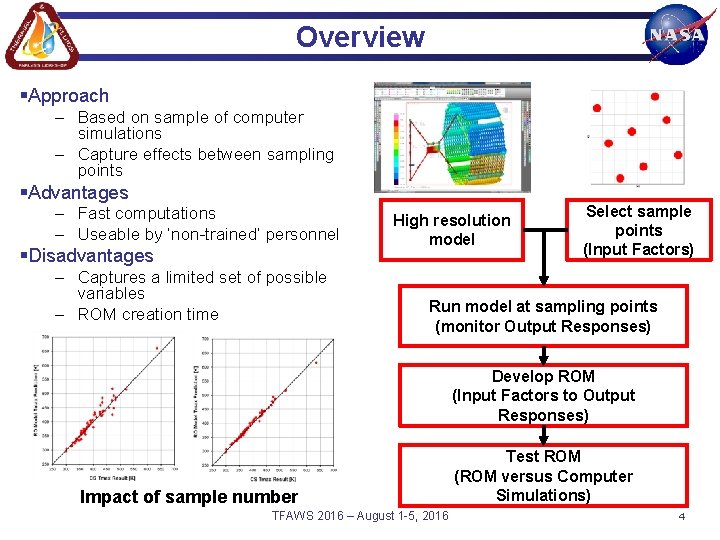
Overview §Approach – Based on sample of computer simulations – Capture effects between sampling points §Advantages – Fast computations – Useable by ‘non-trained’ personnel §Disadvantages – Captures a limited set of possible variables – ROM creation time High resolution model Select sample points (Input Factors) Run model at sampling points (monitor Output Responses) Develop ROM (Input Factors to Output Responses) Impact of sample number TFAWS 2016 – August 1 -5, 2016 Test ROM (ROM versus Computer Simulations) 4

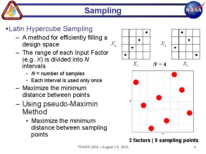
Sampling §Latin Hypercube Sampling – A method for efficiently filling a design space – The range of each Input Factor (e. g. X) is divided into N intervals N=4 • N = number of samples • Each interval is used only once – Maximize the minimum distance between points – Using pseudo-Maximin Method • Maximize the minimum distance between sampling points TFAWS 2016 – August 1 -5, 2016 2 factors | 8 sampling points 5

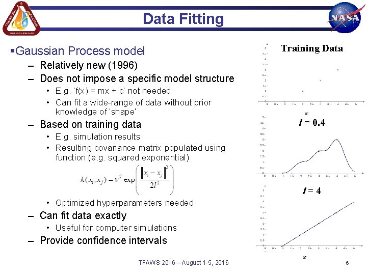
Data Fitting §Gaussian Process model Training Data – Relatively new (1996) – Does not impose a specific model structure • E. g. ‘f(x) = mx + c’ not needed • Can fit a wide-range of data without prior knowledge of ‘shape’ – Based on training data l = 0. 4 • E. g. simulation results • Resulting covariance matrix populated using function (e. g. squared exponential) l=4 • Optimized hyperparameters needed – Can fit data exactly • Useful for computer simulations – Provide confidence intervals TFAWS 2016 – August 1 -5, 2016 6

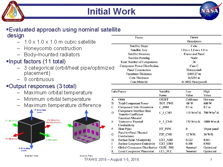
Initial Work §Evaluated approach using nominal satellite design – 1. 0 x 1. 0 m cubic satellite – Honeycomb construction – Body-mounted radiators §Input factors (11 total) – 3 categorical (orbit/heat pipe/optimized placement) – 8 continuous §Output responses (3 total) – Maximum orbital temperature – Minimum orbital temperature – Maximum temperature difference TFAWS 2016 – August 1 -5, 2016 7

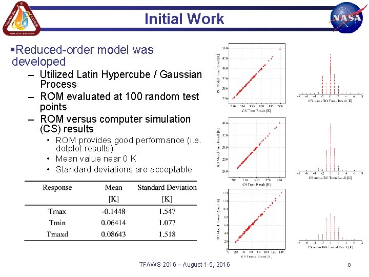
Initial Work §Reduced-order model was developed – Utilized Latin Hypercube / Gaussian Process – ROM evaluated at 100 random test points – ROM versus computer simulation (CS) results • ROM provides good performance (i. e. dotplot results) • Mean value near 0 K • Standard deviations are acceptable TFAWS 2016 – August 1 -5, 2016 8

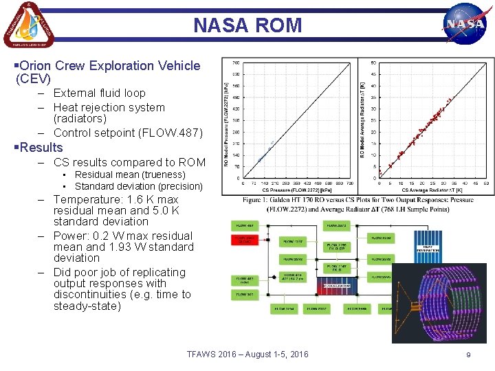
NASA ROM §Orion Crew Exploration Vehicle (CEV) – External fluid loop – Heat rejection system (radiators) – Control setpoint (FLOW. 487) §Results – CS results compared to ROM • Residual mean (trueness) • Standard deviation (precision) – Temperature: 1. 6 K max residual mean and 5. 0 K standard deviation – Power: 0. 2 W max residual mean and 1. 93 W standard deviation – Did poor job of replicating output responses with discontinuities (e. g. time to steady-state) TFAWS 2016 – August 1 -5, 2016 9

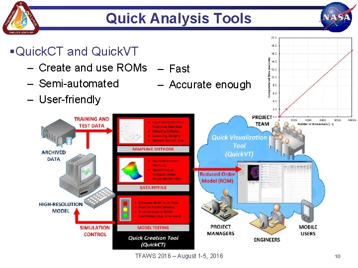
Quick Analysis Tools §Quick. CT and Quick. VT – Create and use ROMs – Fast – Semi-automated – Accurate enough – User-friendly TFAWS 2016 – August 1 -5, 2016 10

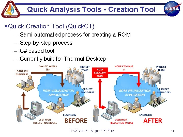
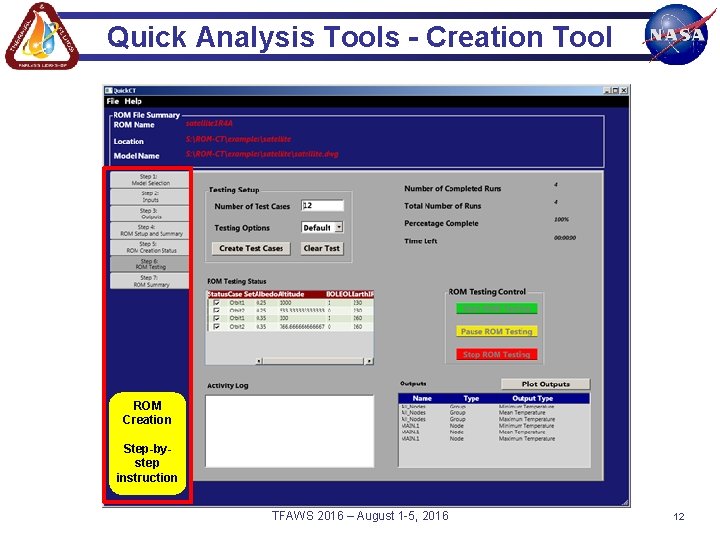
Quick Analysis Tools - Creation Tool §Quick Creation Tool (Quick. CT) – – Semi-automated process for creating a ROM Step-by-step process C# based tool Currently built for Thermal Desktop TFAWS 2016 – August 1 -5, 2016 11

Quick Analysis Tools - Creation Tool ROM Creation Step-bystep instruction TFAWS 2016 – August 1 -5, 2016 12

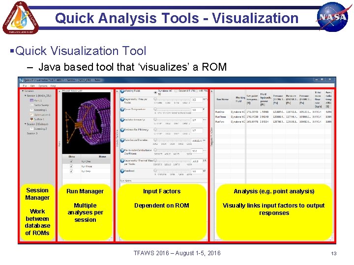
Quick Analysis Tools - Visualization §Quick Visualization Tool – Java based tool that ‘visualizes’ a ROM Session Manager Work between database of ROMs Run Manager Input Factors Analysis (e. g. point analysis) Multiple analyses per session Dependent on ROM Visually links input factors to output responses TFAWS 2016 – August 1 -5, 2016 13

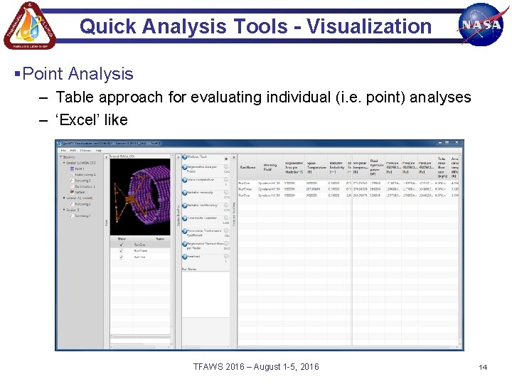
Quick Analysis Tools - Visualization §Point Analysis – Table approach for evaluating individual (i. e. point) analyses – ‘Excel’ like TFAWS 2016 – August 1 -5, 2016 14

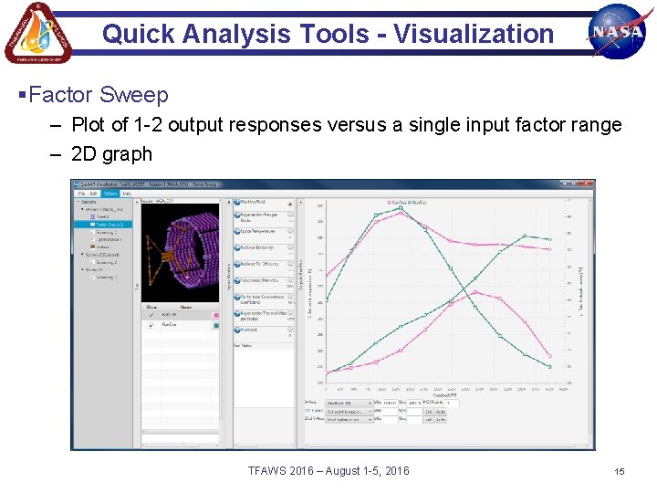
Quick Analysis Tools - Visualization §Factor Sweep – Plot of 1 -2 output responses versus a single input factor range – 2 D graph TFAWS 2016 – August 1 -5, 2016 15

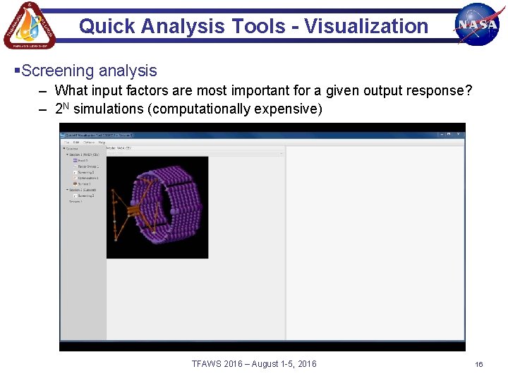
Quick Analysis Tools - Visualization §Screening analysis – What input factors are most important for a given output response? – 2 N simulations (computationally expensive) TFAWS 2016 – August 1 -5, 2016 16

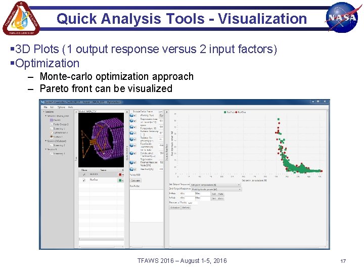
Quick Analysis Tools - Visualization § 3 D Plots (1 output response versus 2 input factors) §Optimization – Monte-carlo optimization approach – Pareto front can be visualized TFAWS 2016 – August 1 -5, 2016 17

Path Forward §Beta test Quick. AT – Quick. CT and Quick. VT §Quick CT – Additional sampling/data fitting features – Develop for other data sources/platforms §Quick VT – Additional analysis capabilities – Add uncertainty to results TFAWS 2016 – August 1 -5, 2016 18