TCP Congestion Control Jennifer Rexford Fall 2016 TTh

TCP Congestion Control Jennifer Rexford Fall 2016 (TTh 3: 00 -4: 20 in CS 105) COS 561: Advanced Computer Networks http: //www. cs. princeton. edu/courses/archive/fall 16/cos 561/

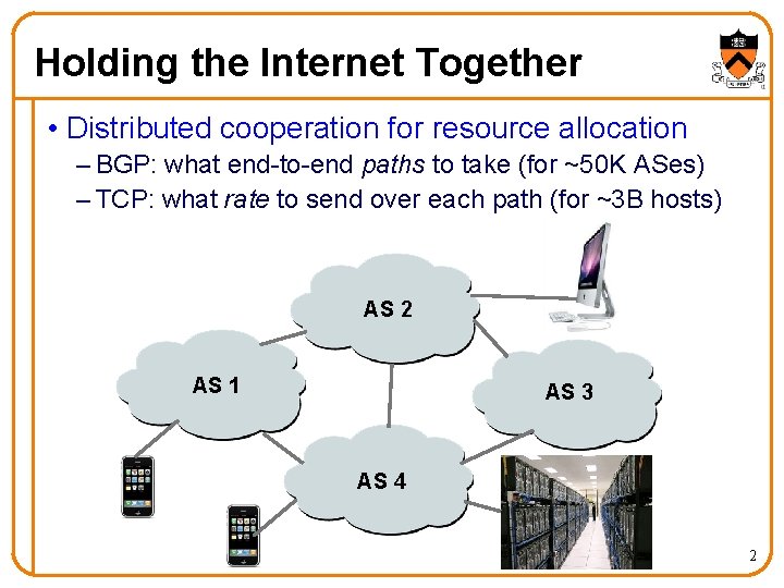
Holding the Internet Together • Distributed cooperation for resource allocation – BGP: what end-to-end paths to take (for ~50 K ASes) – TCP: what rate to send over each path (for ~3 B hosts) AS 2 AS 1 AS 3 AS 4 2

What Problem Does a Protocol Solve? • BGP path selection – Select a path that each AS on the path is willing to use – Adapt path selection in the presence of failures • TCP congestion control – Prevent congestion collapse of the Internet – Allocate bandwidth fairly and efficiently • But, can we be more precise? – Define mathematically what problem is being solved – To understand the problem and analyze the protocol – To predict the effects of changes in the system – To design better protocols from first principles 3

Fairness 4

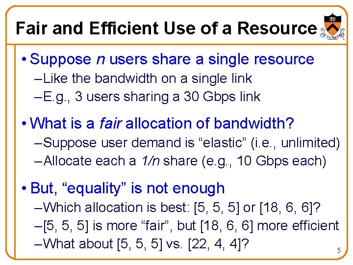
Fair and Efficient Use of a Resource • Suppose n users share a single resource – Like the bandwidth on a single link – E. g. , 3 users sharing a 30 Gbps link • What is a fair allocation of bandwidth? – Suppose user demand is “elastic” (i. e. , unlimited) – Allocate each a 1/n share (e. g. , 10 Gbps each) • But, “equality” is not enough – Which allocation is best: [5, 5, 5] or [18, 6, 6]? – [5, 5, 5] is more “fair”, but [18, 6, 6] more efficient – What about [5, 5, 5] vs. [22, 4, 4]? 5

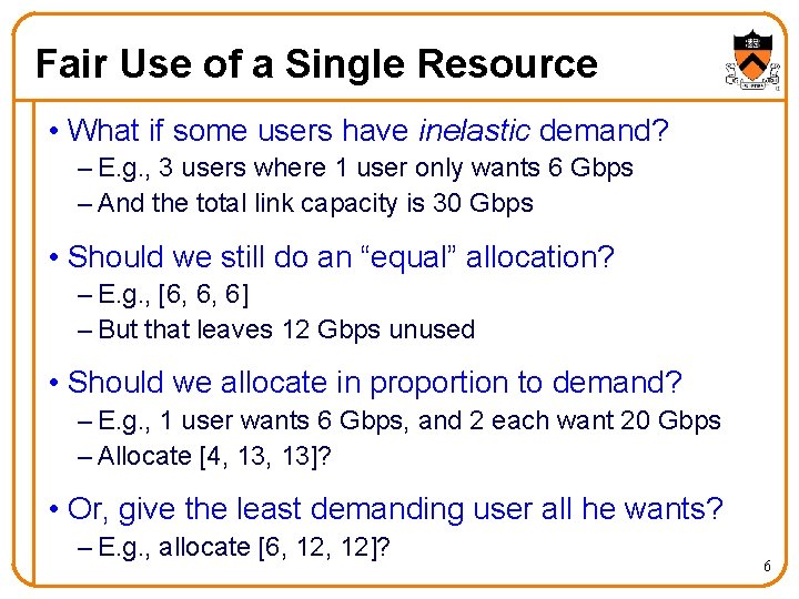
Fair Use of a Single Resource • What if some users have inelastic demand? – E. g. , 3 users where 1 user only wants 6 Gbps – And the total link capacity is 30 Gbps • Should we still do an “equal” allocation? – E. g. , [6, 6, 6] – But that leaves 12 Gbps unused • Should we allocate in proportion to demand? – E. g. , 1 user wants 6 Gbps, and 2 each want 20 Gbps – Allocate [4, 13]? • Or, give the least demanding user all he wants? – E. g. , allocate [6, 12]? 6

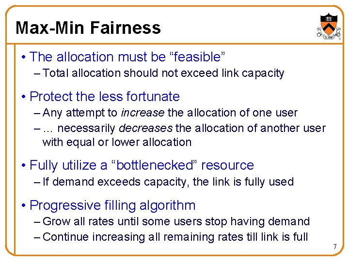
Max-Min Fairness • The allocation must be “feasible” – Total allocation should not exceed link capacity • Protect the less fortunate – Any attempt to increase the allocation of one user – … necessarily decreases the allocation of another user with equal or lower allocation • Fully utilize a “bottlenecked” resource – If demand exceeds capacity, the link is fully used • Progressive filling algorithm – Grow all rates until some users stop having demand – Continue increasing all remaining rates till link is full 7

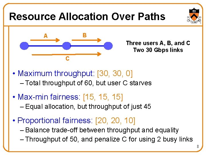
Resource Allocation Over Paths B A Three users A, B, and C Two 30 Gbps links C • Maximum throughput: [30, 0] – Total throughput of 60, but user C starves • Max-min fairness: [15, 15] – Equal allocation, but throughput of just 45 • Proportional fairness: [20, 10] – Balance trade-off between throughput and equality – Throughput of 50, and penalize C for using 2 busy links 8

Distributed Algorithm for Achieving Fairness 9

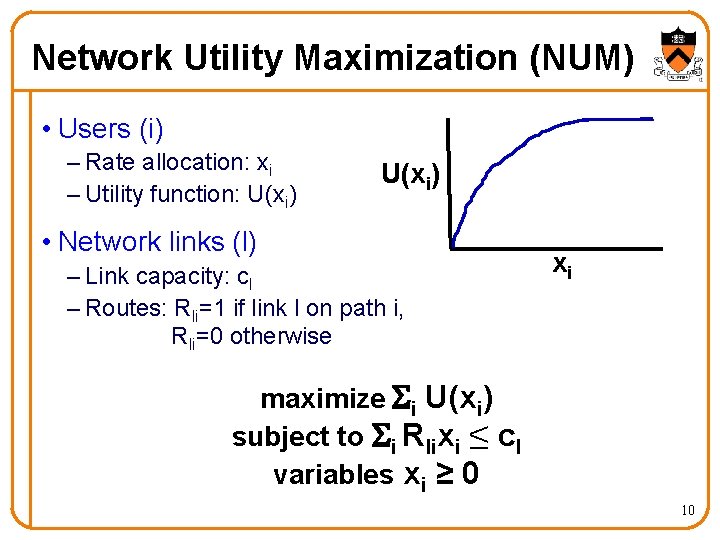
Network Utility Maximization (NUM) • Users (i) – Rate allocation: xi – Utility function: U(xi) • Network links (l) – Link capacity: cl – Routes: Rli=1 if link l on path i, Rli=0 otherwise xi maximize Si U(xi) subject to Si Rlixi ≤ cl variables xi ≥ 0 10

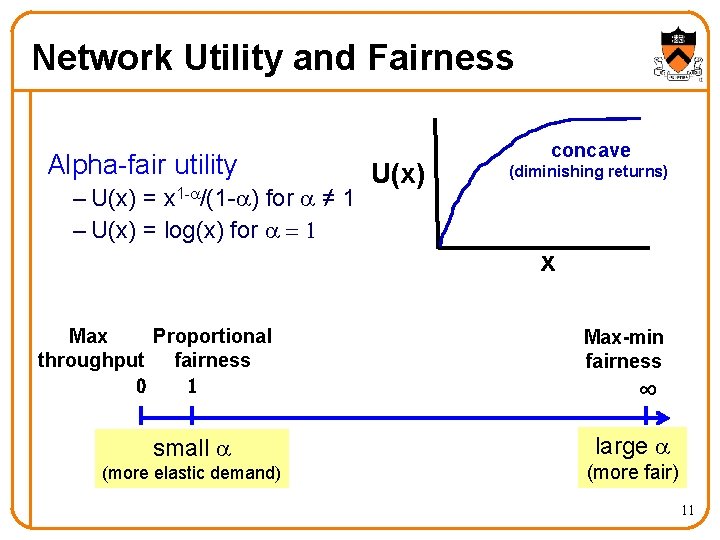
Network Utility and Fairness Alpha-fair utility – U(x) = x 1 -a/(1 -a) for a ≠ 1 – U(x) = log(x) for a = 1 U(x) concave (diminishing returns) x Max Proportional throughput fairness 0 1 small a (more elastic demand) Max-min fairness ∞ large a (more fair) 11

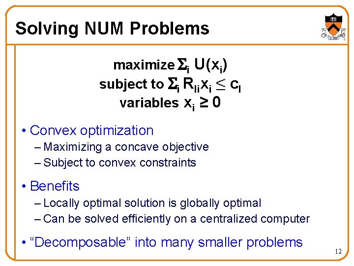
Solving NUM Problems maximize Si U(xi) subject to Si Rlixi ≤ cl variables xi ≥ 0 • Convex optimization – Maximizing a concave objective – Subject to convex constraints • Benefits – Locally optimal solution is globally optimal – Can be solved efficiently on a centralized computer • “Decomposable” into many smaller problems 12

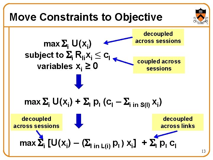
Move Constraints to Objective max Si U(xi) subject to Si Rlixi ≤ cl variables xi ≥ 0 decoupled across sessions max Si U(xi) + Sl pl (cl – Si in S(l) xi) decoupled across sessions decoupled across links max Si [U(xi) – (Sl in L(i) pl ) xi] + Sl pl cl 13

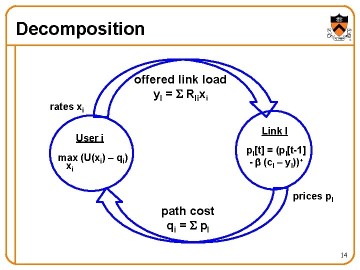
Decomposition rates xi offered link load yl = S Rlixi Link l User i pl[t] = (pl[t-1] - b (cl – yl))+ max (U(xi) – qi) xi prices pl path cost qi = S pl 14

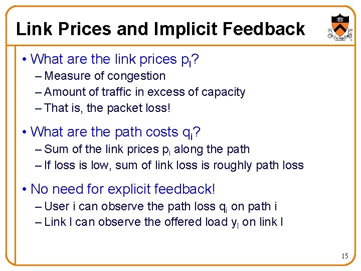
Link Prices and Implicit Feedback • What are the link prices pl? – Measure of congestion – Amount of traffic in excess of capacity – That is, the packet loss! • What are the path costs qi? – Sum of the link prices pl along the path – If loss is low, sum of link loss is roughly path loss • No need for explicit feedback! – User i can observe the path loss qi on path i – Link l can observe the offered load yl on link l 15

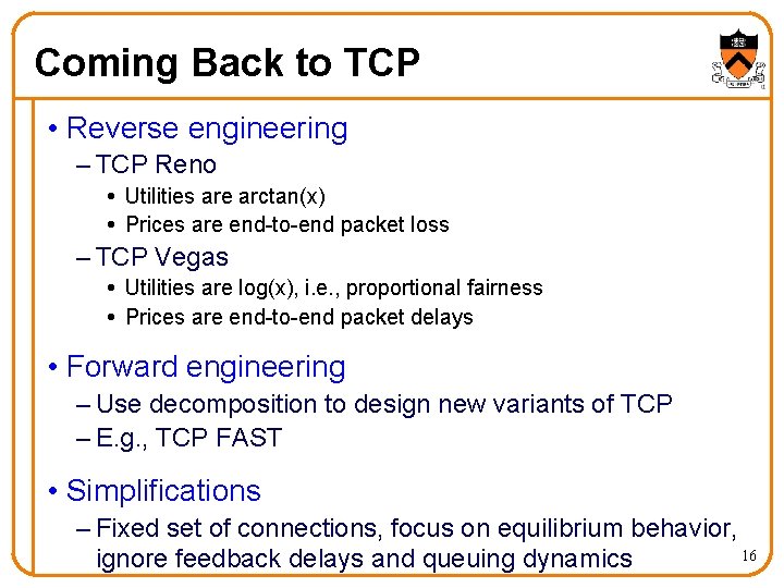
Coming Back to TCP • Reverse engineering – TCP Reno Utilities are arctan(x) Prices are end-to-end packet loss – TCP Vegas Utilities are log(x), i. e. , proportional fairness Prices are end-to-end packet delays • Forward engineering – Use decomposition to design new variants of TCP – E. g. , TCP FAST • Simplifications – Fixed set of connections, focus on equilibrium behavior, 16 ignore feedback delays and queuing dynamics

TCP Congestion Control 17

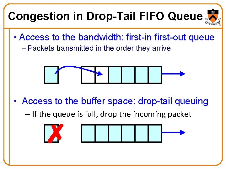
Congestion in Drop-Tail FIFO Queue • Access to the bandwidth: first-in first-out queue – Packets transmitted in the order they arrive • Access to the buffer space: drop-tail queuing – If the queue is full, drop the incoming packet ✗

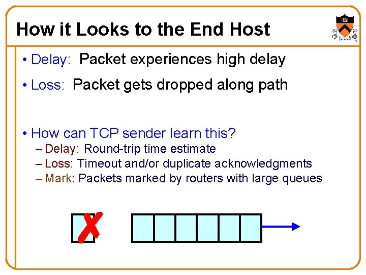
How it Looks to the End Host • Delay: Packet experiences high delay • Loss: Packet gets dropped along path • How can TCP sender learn this? – Delay: Round-trip time estimate – Loss: Timeout and/or duplicate acknowledgments – Mark: Packets marked by routers with large queues ✗

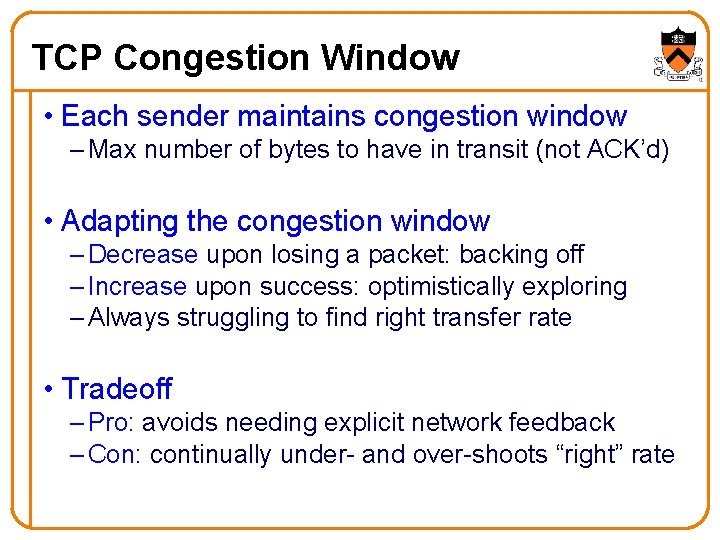
TCP Congestion Window • Each sender maintains congestion window – Max number of bytes to have in transit (not ACK’d) • Adapting the congestion window – Decrease upon losing a packet: backing off – Increase upon success: optimistically exploring – Always struggling to find right transfer rate • Tradeoff – Pro: avoids needing explicit network feedback – Con: continually under- and over-shoots “right” rate

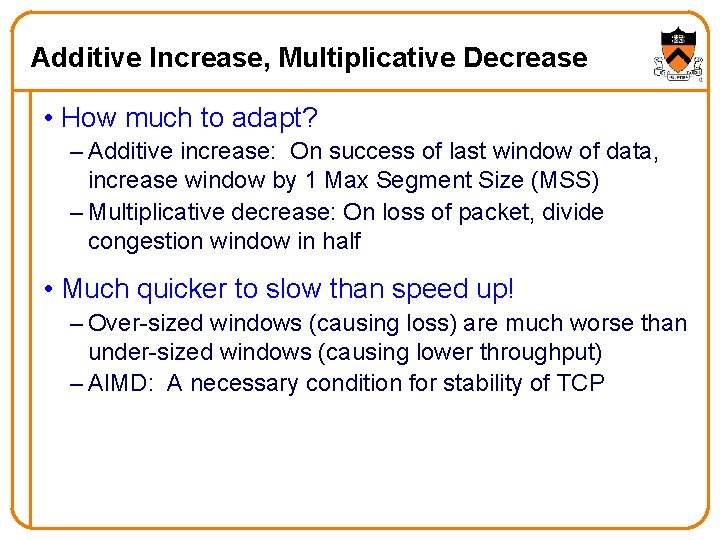
Additive Increase, Multiplicative Decrease • How much to adapt? – Additive increase: On success of last window of data, increase window by 1 Max Segment Size (MSS) – Multiplicative decrease: On loss of packet, divide congestion window in half • Much quicker to slow than speed up! – Over-sized windows (causing loss) are much worse than under-sized windows (causing lower throughput) – AIMD: A necessary condition for stability of TCP

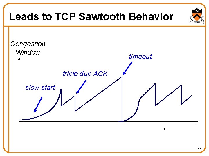
Leads to TCP Sawtooth Behavior Congestion Window timeout triple dup ACK slow start t 22

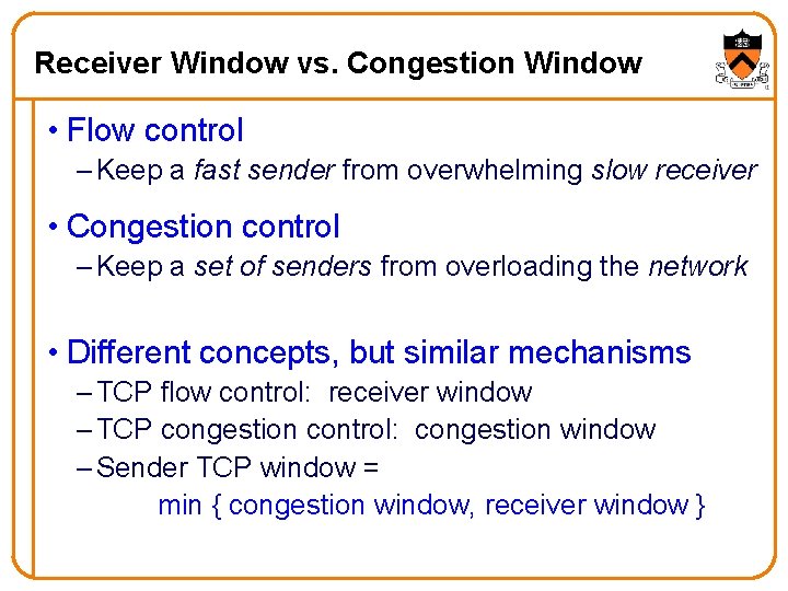
Receiver Window vs. Congestion Window • Flow control – Keep a fast sender from overwhelming slow receiver • Congestion control – Keep a set of senders from overloading the network • Different concepts, but similar mechanisms – TCP flow control: receiver window – TCP congestion control: congestion window – Sender TCP window = min { congestion window, receiver window }

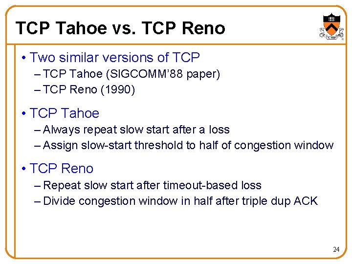
TCP Tahoe vs. TCP Reno • Two similar versions of TCP – TCP Tahoe (SIGCOMM’ 88 paper) – TCP Reno (1990) • TCP Tahoe – Always repeat slow start after a loss – Assign slow-start threshold to half of congestion window • TCP Reno – Repeat slow start after timeout-based loss – Divide congestion window in half after triple dup ACK 24

Discussion 25