Statistical Learning with Application of R Prayrie Sinha

Statistical Learning with Application of R Prayrie Sinha Summer Trainee

R � R is a programming language and free software environment for statistical computing and graphics that is supported by the R Foundation for Statistical Computing. The R language is widely used among statisticians and data miners for developing statistical software and data analysis. The source code for the R software environment is written primarily in C, Fortran, and R.

CONTENTS � � � � What is Statistical Learning? Linear Regression Classification Resampling Methods Linear Model Selection and Regularization Decision Trees Clustering

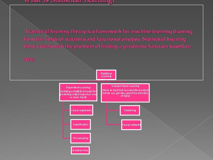
What is Statistical Learning? Statistical learning theory is a framework for machine learning drawing from the fields of statistics and functional analysis. Statistical learning theory deals with the problem of finding a predictive function based on data. Statistical Learning Supervised Learning (building a statistical model for predicting output based on one or more input) Linear regression Classification Re-sampling Decision tree Unsupervised Learning (there is input but no supervised output but we can get idea about the structure of data) Clustering Neural networks

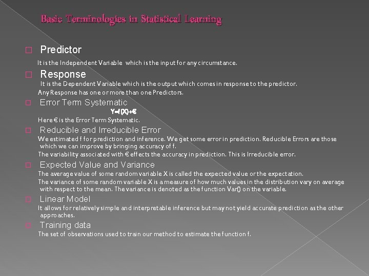
Basic Terminologies in Statistical Learning � Predictor It is the Independent Variable which is the input for any circumstance. � Response It is the Dependent Variable which is the output which comes in response to the predictor. Any Response has one or more than one Predictors. � Error Term Systematic Y=f(X)+€ Here € is the Error Term Systematic. � Reducible and Irreducible Error We estimated f for prediction and inference. We get some error in prediction. Reducible Errors are those which we can improve by bringing accuracy of f. The variability associated with € effects the accuracy in prediction. This is Irreducible error. � Expected Value and Variance The average value of some random variable X is called the expected value or the expectation. The variance of some random variable X is a measure of how much values in the distribution vary on average with respect to the mean. The variance is denoted as the function Var() on the variable. � Linear Model It allows for relatively simple and interpretable inference but may not yield accurate prediction as the other approaches. � Training data The set of observations used to train our method to estimate the function f.

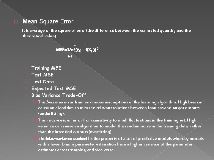
� Mean Square Error It is average of the square of error(the difference between the estimated quantity and theoretical value) n ^ MSE=1/n∑(yi - f(Xi )) 2 i=1 › › › Training MSE Test Data Expected Test MSE Bias Variance Trade-Off � The bias is an error from erroneous assumptions in the learning algorithm. High bias can cause an algorithm to miss the relevant relations between features and target outputs (underfitting). � The variance is an error from sensitivity to small fluctuations in the training set. High variance can cause an algorithm to model the random noise in the training data, rather than the intended outputs (overfitting). � the bias–variance tradeoff is the property of a set of predictive models whereby models with a lower bias in parameter estimation have a higher variance of the parameter estimates across samples, and vice versa.

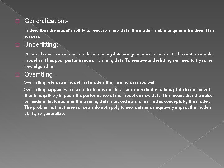
� Generalization: It describes the model’s ability to react to a new data. If a model is able to generalize then it is a success. � Underfitting: A model which can neither model a training data nor generalize to new data. It is not a suitable model as it has poor performance on training data. To remove underfitting we need to try some new algorithm. � Overfitting: Overfitting refers to a model that models the training data too well. Overfitting happens when a model learns the detail and noise in the training data to the extent that it negatively impacts the performance of the model on new data. This means that the noise or random fluctuations in the training data is picked up and learned as concepts by the model. The problem is that these concepts do not apply to new data and negatively impact the models ability to generalize.

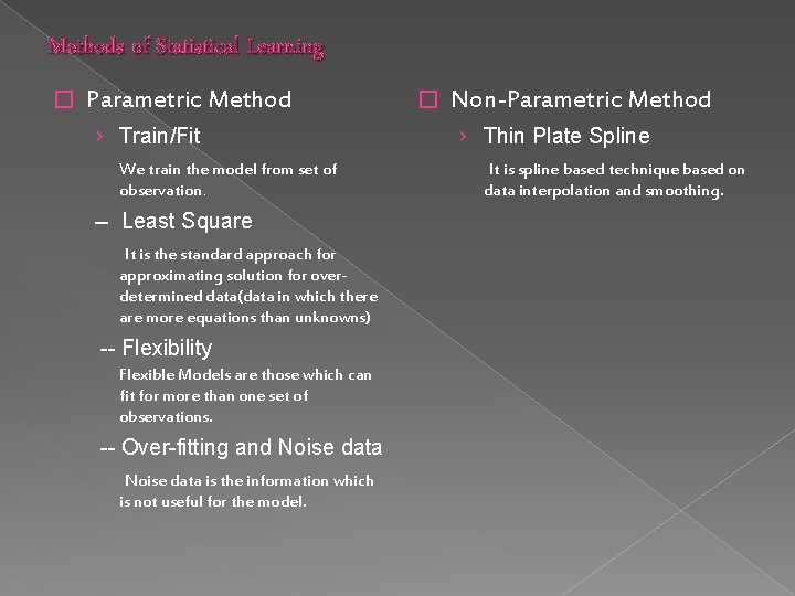
Methods of Statistical Learning � Parametric Method › Train/Fit We train the model from set of observation. -- Least Square It is the standard approach for approximating solution for overdetermined data(data in which there are more equations than unknowns) -- Flexibility Flexible Models are those which can fit for more than one set of observations. -- Over-fitting and Noise data is the information which is not useful for the model. � Non-Parametric Method › Thin Plate Spline It is spline based technique based on data interpolation and smoothing.

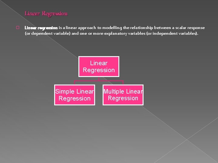
Linear Regression � Linear regression is a linear approach to modelling the relationship between a scalar response (or dependent variable) and one or more explanatory variables (or independent variables). Linear Regression Simple Linear Regression Multiple Linear Regression

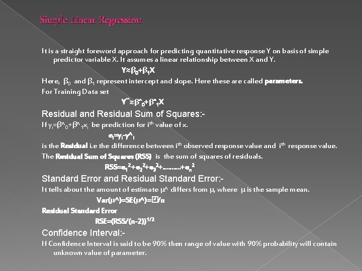
Simple Linear Regression It is a straight foreword approach for predicting quantitative response Y on basis of simple predictor variable X. It assumes a linear relationship between X and Y. Y≈β 0+β 1 X Here, β 0 and β 1 represent intercept and slope. Here these are called parameters. For Training Data set Yˆˆ≈βˆ0+βˆ1 X Residual and Residual Sum of Squares: If yi=β^0+β^1 xi be prediction for ith value of x. ei=yi-y^i is the Residual i. e the difference between ith observed response value and ith response value. The Residual Sum of Squares (RSS) is the sum of squares of residuals. RSS=e 12 +e 22+e 32+………. +en 2 Standard Error and Residual Standard Error: It tells about the amount of estimate μ^ differs from μ, where μ is the sample mean. 2 /n Var(μ^)=SE(μ^)=� Residual Standard Error RSE=(RSS/(n-2))1/2 Confidence Interval: If Confidence Interval is said to be 90% then range of value with 90% probability will contain unknown value of parameter.

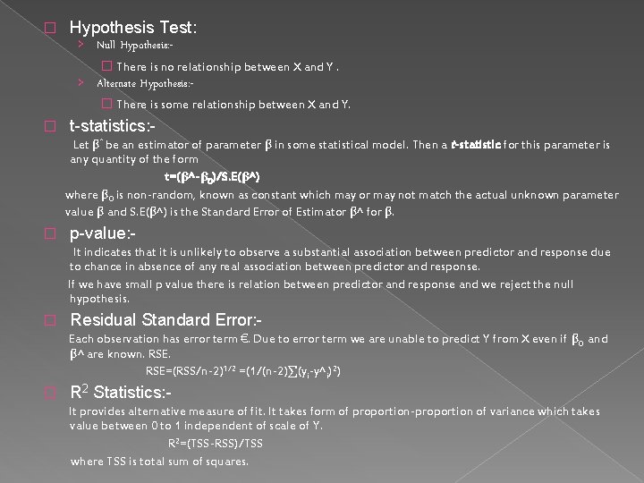
� Hypothesis Test: › Null Hypothesis: - � There is no relationship between X and Y. › Alternate Hypothesis: - � There is some relationship between X and Y. � t-statistics: - Let βˆ be an estimator of parameter β in some statistical model. Then a t-statistic for this parameter is any quantity of the form t=(β^-β 0)/S. E(β^) where β 0 is non-random, known as constant which may or may not match the actual unknown parameter value β and S. E(β^) is the Standard Error of Estimator β^ for β. � p-value: - It indicates that it is unlikely to observe a substantial association between predictor and response due to chance in absence of any real association between predictor and response. If we have small p value there is relation between predictor and response and we reject the null hypothesis. � Residual Standard Error: - Each observation has error term €. Due to error term we are unable to predict Y from X even if β 0 and β^ are known. RSE. RSE=(RSS/n-2)1/2 =(1/(n-2)∑(yi-y^i)2) � R 2 Statistics: - It provides alternative measure of fit. It takes form of proportion-proportion of variance which takes value between 0 to 1 independent of scale of Y. R 2=(TSS-RSS)/TSS where TSS is total sum of squares.

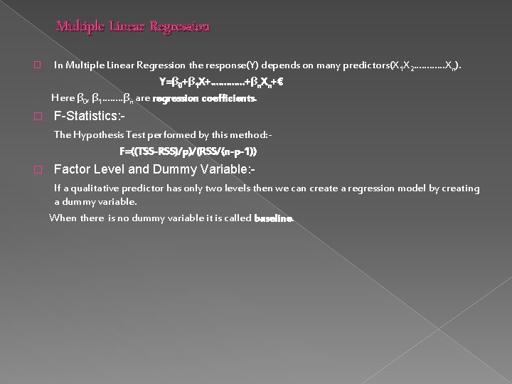
Multiple Linear Regression In Multiple Linear Regression the response(Y) depends on many predictors(X 1 X 2…………Xn). Y=β 0+β 1 X+…………. +βn. Xn+€ Here β 0, β 1……. . βn are regression coefficients. � � F-Statistics: - The Hypothesis Test performed by this method: F=((TSS-RSS)/p)/(RSS/(n-p-1)) � Factor Level and Dummy Variable: - If a qualitative predictor has only two levels then we can create a regression model by creating a dummy variable. When there is no dummy variable it is called baseline.

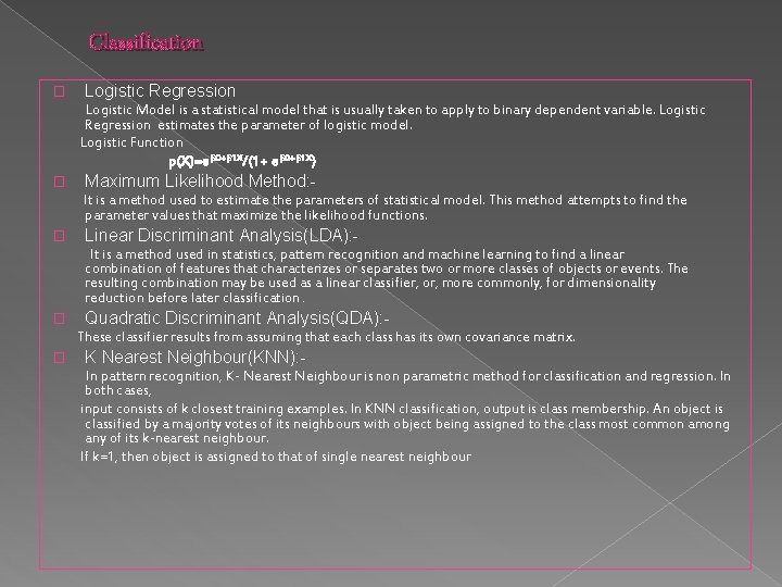
Classification Logistic Regression � Logistic Model is a statistical model that is usually taken to apply to binary dependent variable. Logistic Regression estimates the parameter of logistic model. Logistic Function p(X)=eβ 0+β 1 X/(1+ eβ 0+β 1 X) � Maximum Likelihood Method: It is a method used to estimate the parameters of statistical model. This method attempts to find the parameter values that maximize the likelihood functions. � Linear Discriminant Analysis(LDA): It is a method used in statistics, pattern recognition and machine learning to find a linear combination of features that characterizes or separates two or more classes of objects or events. The resulting combination may be used as a linear classifier, or, more commonly, for dimensionality reduction before later classification. � Quadratic Discriminant Analysis(QDA): These classifier results from assuming that each class has its own covariance matrix. � K Nearest Neighbour(KNN): In pattern recognition, K- Nearest Neighbour is non parametric method for classification and regression. In both cases, input consists of k closest training examples. In KNN classification, output is class membership. An object is classified by a majority votes of its neighbours with object being assigned to the class most common among any of its k-nearest neighbour. If k=1, then object is assigned to that of single nearest neighbour

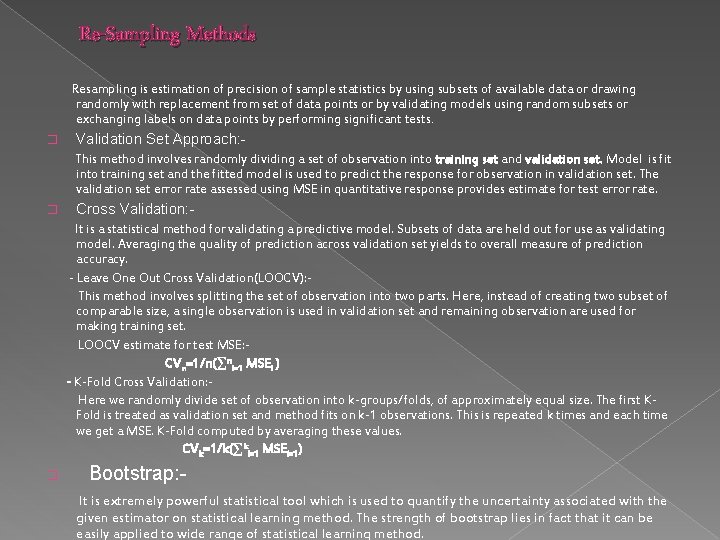
Re-Sampling Methods Resampling is estimation of precision of sample statistics by using subsets of available data or drawing randomly with replacement from set of data points or by validating models using random subsets or exchanging labels on data points by performing significant tests. � Validation Set Approach: This method involves randomly dividing a set of observation into training set and validation set. Model is fit into training set and the fitted model is used to predict the response for observation in validation set. The validation set error rate assessed using MSE in quantitative response provides estimate for test error rate. � Cross Validation: - It is a statistical method for validating a predictive model. Subsets of data are held out for use as validating model. Averaging the quality of prediction across validation set yields to overall measure of prediction accuracy. - Leave One Out Cross Validation(LOOCV): This method involves splitting the set of observation into two parts. Here, instead of creating two subset of comparable size, a single observation is used in validation set and remaining observation are used for making training set. LOOCV estimate for test MSE: CVn=1/n(∑ni=1 MSEi ) - K-Fold Cross Validation: Here we randomly divide set of observation into k-groups/folds, of approximately equal size. The first KFold is treated as validation set and method fits on k-1 observations. This is repeated k times and each time we get a MSE. K-Fold computed by averaging these values. CVk=1/k(∑ki=1 MSEi=1) � Bootstrap: It is extremely powerful statistical tool which is used to quantify the uncertainty associated with the given estimator on statistical learning method. The strength of bootstrap lies in fact that it can be easily applied to wide range of statistical learning method.

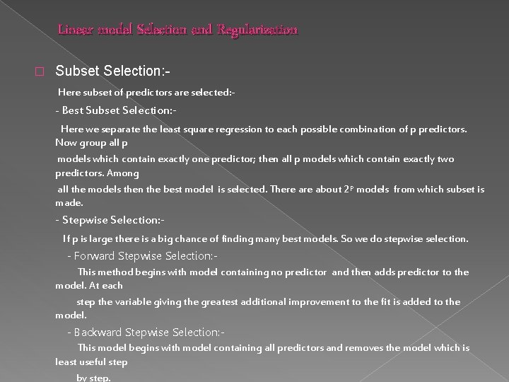
Linear model Selection and Regularization � Subset Selection: Here subset of predictors are selected: - - Best Subset Selection: - Here we separate the least square regression to each possible combination of p predictors. Now group all p models which contain exactly one predictor; then all p models which contain exactly two predictors. Among all the models then the best model is selected. There about 2 p models from which subset is made. - Stepwise Selection: - If p is large there is a big chance of finding many best models. So we do stepwise selection. - Forward Stepwise Selection: This method begins with model containing no predictor and then adds predictor to the model. At each step the variable giving the greatest additional improvement to the fit is added to the model. - Backward Stepwise Selection: This model begins with model containing all predictors and removes the model which is least useful step by step.

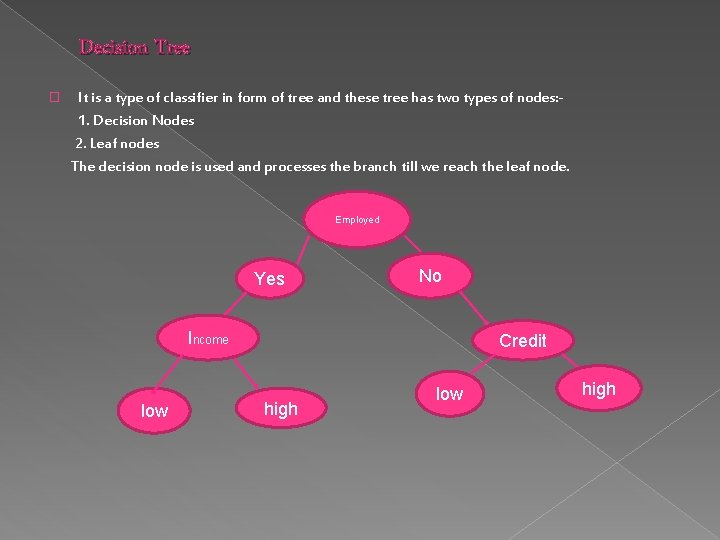
Decision Tree It is a type of classifier in form of tree and these tree has two types of nodes: 1. Decision Nodes 2. Leaf nodes The decision node is used and processes the branch till we reach the leaf node. � Employed Yes No Income low Credit high low high

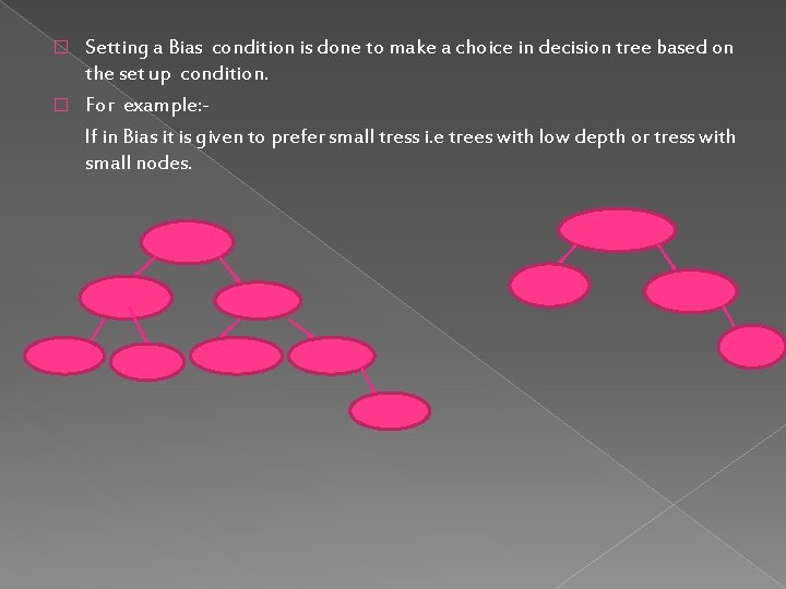
Setting a Bias condition is done to make a choice in decision tree based on the set up condition. � For example: If in Bias it is given to prefer small tress i. e trees with low depth or tress with small nodes. �

Clustering is a part of Unsupervised learning. � Clustering is task of grouping set of objects in such a way that objects with same group are more similar to each other than the groups of other clusters. � It is useful for: � › Automatically organizing data. › Understanding the hidden structure in data. › Preprocessing for further analysis � Aspects of Clustering: - Quality of Clustering depends on the: - Algorithm: Partition Clustering: - Here various partitions are constructed and then evaluate by some criterions. For Example: - k means. Hierarchical Clustering : - Create hierarchical decomposition of the set of objects using some criterion.

- Distance or Similarity Functions: - To get how similar or dissimilar two clusters are we use Euclidean Function , Cosine Function. Clustering Quality: Used to see how good the clustering is done. - Inter Clustering Distance: - We maximize the inter clustered distance so that different clusters stay far apart. Intra Clustering Distance: - We minimize the distance between the elements of the same cluster.

Thank You.