SelfOrganizing Lists Competitive Analysis Lee Wee Sun So

Self-Organizing Lists Competitive Analysis Lee Wee Sun So. C 1 5 -26 leews@comp. nus. edu. sg Modified by Orgad Keller Modified again by Ariel Rosenfeld Self-Organizing Lists 1

Self-Organizing List • List L of n elements – Operations Access(x) cost rank(x)=position of x in the list – L can be reordered by transposing adjacent elements – cost = 1. Self-Organizing Lists 2

On-line Problem • Problem: Sequence S of operations to which the algorithm must respond to without knowing the future inputs. • Goal: Minimize the total cost of responding to the operations. • Ignore computational cost except for access and reorder Self-Organizing Lists 3

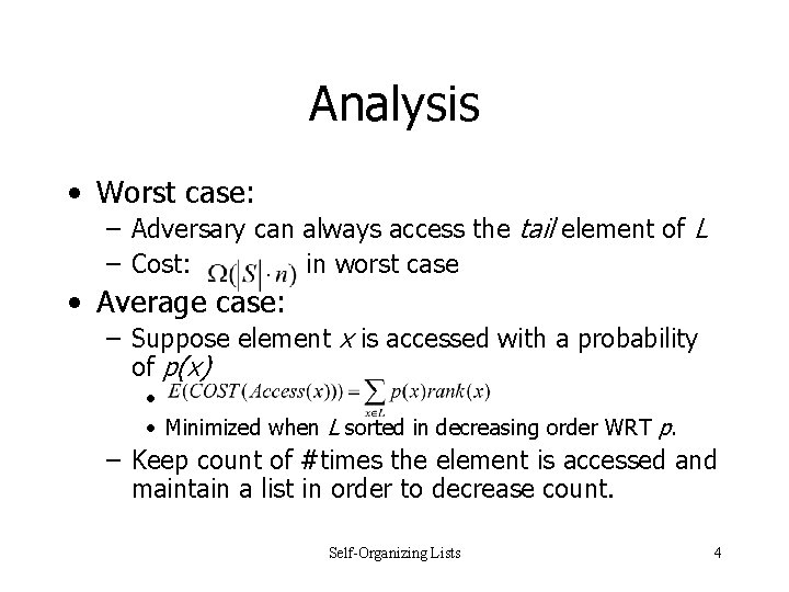
Analysis • Worst case: – Adversary can always access the tail element of L – Cost: in worst case • Average case: – Suppose element x is accessed with a probability of p(x) • • Minimized when L sorted in decreasing order WRT p. – Keep count of #times the element is accessed and maintain a list in order to decrease count. Self-Organizing Lists 4

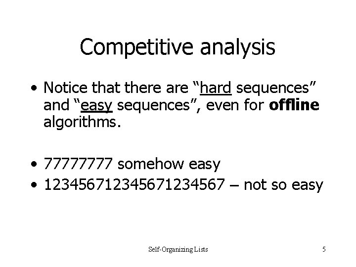
Competitive analysis • Notice that there are “hard sequences” and “easy sequences”, even for offline algorithms. • 7777 somehow easy • 12345671234567 – not so easy Self-Organizing Lists 5

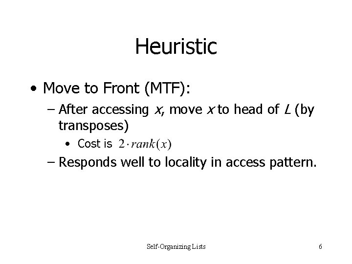
Heuristic • Move to Front (MTF): – After accessing x, move x to head of L (by transposes) • Cost is – Responds well to locality in access pattern. Self-Organizing Lists 6

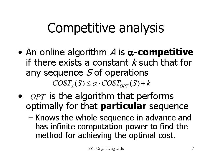
Competitive analysis • An online algorithm A is -competitive if there exists a constant k such that for any sequence S of operations • is the algorithm that performs optimally for that particular sequence – Knows the whole sequence in advance and has infinite computation power to find the method for achieving the optimal cost. Self-Organizing Lists 7

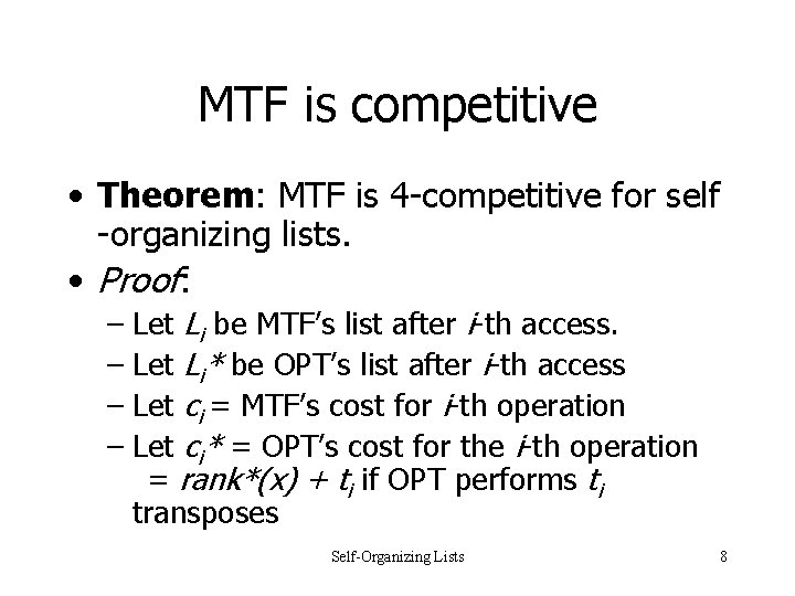
MTF is competitive • Theorem: MTF is 4 -competitive for self -organizing lists. • Proof: – Let Li be MTF’s list after i-th access. – Let Li* be OPT’s list after i-th access – Let ci = MTF’s cost for i-th operation – Let ci* = OPT’s cost for the i-th operation = rank*(x) + ti if OPT performs ti transposes Self-Organizing Lists 8

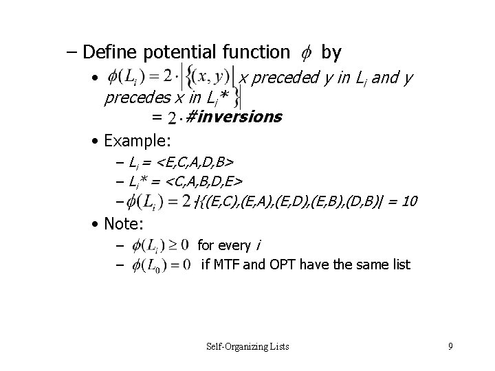
– Define potential function • by x preceded y in Li and y precedes x in Li* = #inversions • Example: – Li = <E, C, A, D, B> – Li* = <C, A, B, D, E> – |{(E, C), (E, A), (E, D), (E, B), (D, B)| = 10 • Note: – – for every i if MTF and OPT have the same list Self-Organizing Lists 9

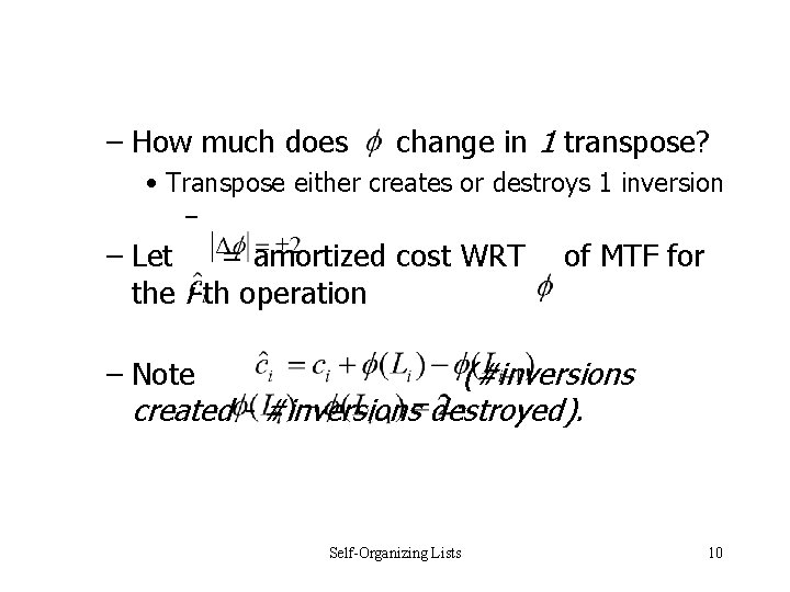
– How much does change in 1 transpose? • Transpose either creates or destroys 1 inversion – – Let = amortized cost WRT the i-th operation of MTF for – Note (#inversions created - #inversions destroyed). Self-Organizing Lists 10

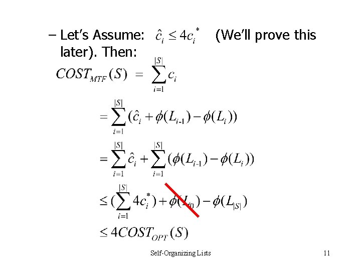
– Let’s Assume: later). Then: (We’ll prove this Self-Organizing Lists 11

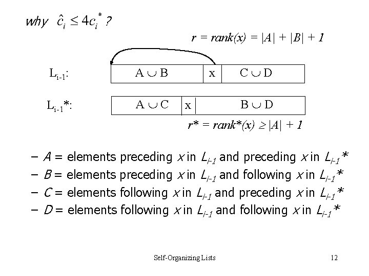
why ? r = rank(x) = |A| + |B| + 1 Li-1: A B Li-1*: A C x x C D B D r* = rank*(x) |A| + 1 – – A = elements preceding x in Li-1 and preceding x in Li-1* B = elements preceding x in Li-1 and following x in Li-1* C = elements following x in Li-1 and preceding x in Li-1* D = elements following x in Li-1 and following x in Li-1* Self-Organizing Lists 12

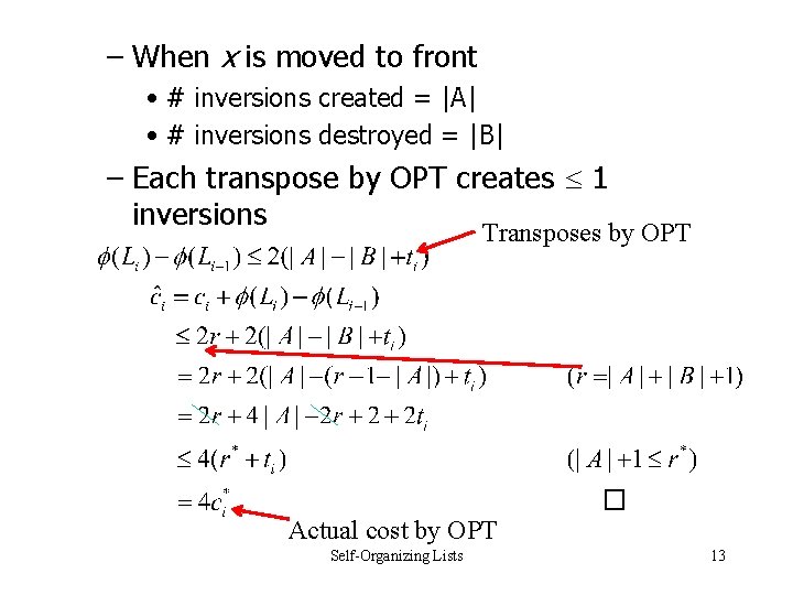
– When x is moved to front • # inversions created = |A| • # inversions destroyed = |B| – Each transpose by OPT creates 1 inversions Transposes by OPT � Actual cost by OPT Self-Organizing Lists 13

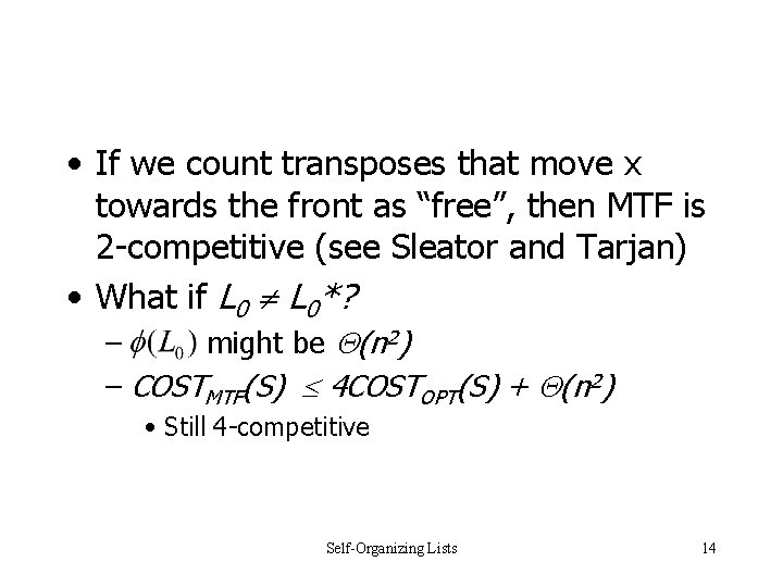
• If we count transposes that move x towards the front as “free”, then MTF is 2 -competitive (see Sleator and Tarjan) • What if L 0*? – might be (n 2) – COSTMTF(S) 4 COSTOPT(S) + (n 2) • Still 4 -competitive Self-Organizing Lists 14

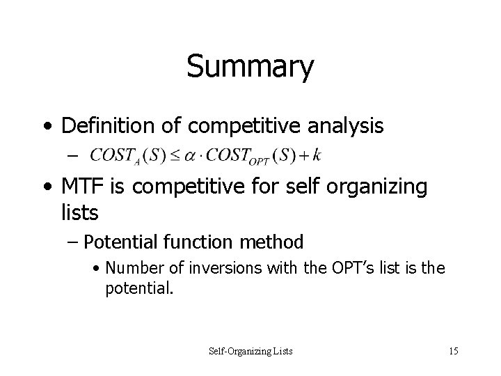
Summary • Definition of competitive analysis – • MTF is competitive for self organizing lists – Potential function method • Number of inversions with the OPT’s list is the potential. Self-Organizing Lists 15