Research and Development Chapter 22 Research and Development

Research and Development Chapter 22: Research and Development 1

Introduction • Technical progress is the source of rising living standards over time • Introduces new concept of efficiency – Static efficiency—traditional allocation of resources to produce existing goods and services so as to maximize surplus and minimize deadweight loss – Dynamic efficiency—creation of new goods and services to raise potential surplus over time • Schumpeterian hypotheses (conflict between static and dynamic efficiency) – Concentrated industries do more research and development of new goods and services, i. e. , are more dynamically efficient, than competitively structured industries – Large firms do more research & development than small firms Chapter 22: Research and Development 2

A Taxonomy of Innovations Product versus Process Innovations • Product Innovations refer to the creation of new goods and new services, e. g. , DVD’s, PDA’s, and cell phones • Process Innovations refer to the development of new technologies for producing goods or new ways of delivering services, e. g. , robotics and CAD/CAM technology • We mainly focus on process or cost-savings innovations but the lines of distinction are blurred—a new product can be the means of implementing a new process Drastic versus Non-Drastic Innovations • Process innovations have two further categories • Drastic innovations have such great cost savings that they permit the innovator to price as an unconstrained monopolist • Non-drastic innovations give the innovator a cost adavantage but not unconstrained monopoly power Chapter 22: Research and Development 3

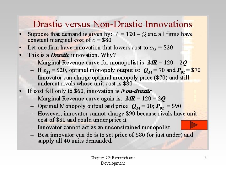
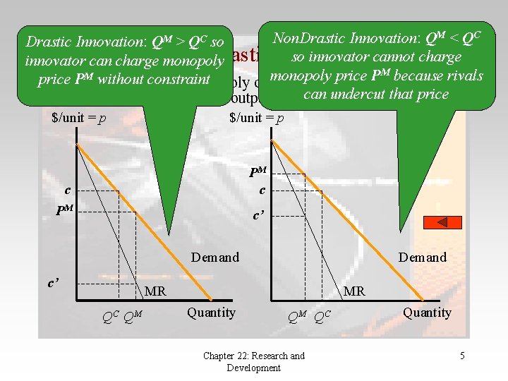
Drastic versus Non-Drastic Innovations • Suppose that demand is given by: P = 120 – Q and all firms have constant marginal cost of c = $80 • Let one firm have innovation that lowers cost to c. M = $20 • This is a Drastic innovation. Why? – Marginal Revenue curve for monopolist is: MR = 120 – 2 Q – If c. M = $20, optimal monopoly output is: QM = 70 and PM = $70 – Innovator can charge optimal monopoly price ($70) and still undercut rivals whose unit cost is $80 • If cost fell only to $60, innovation is Non-drastic – Marginal Revenue curve again is: MR = 120 = 2 Q – Optimal Monopoly output and price: QM = 30; PM = $90 – However, innovator cannot charge $90 because rivals have unit cost of $80 and could under price it – Innovator cannot act as an unconstrained monopolist – Best innovator can do is to set price of $80 (or just under) and supply all 40 units demanded. Chapter 22: Research and Development 4

Non. Drastic Innovation: QM < QC Drastic Innovation: QM > QC so Drastic vs. Non-Drastic Innovations (cont. ) so innovator cannot charge innovator can charge monopoly M because rivals M without constraint monopoly price P M price P Innovation is drastic if monopoly output Q at MR = new marginal c’ exceeds the competitive output QC atcan oldundercut marginalthat costprice c $/unit = p c PM c’ Demand MR QC QM MR Quantity QM QC Chapter 22: Research and Development Quantity 5

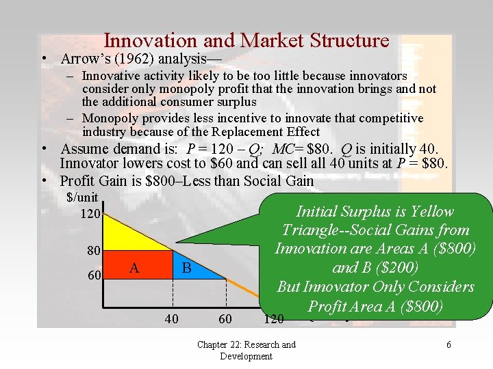
Innovation and Market Structure • Arrow’s (1962) analysis— – Innovative activity likely to be too little because innovators consider only monopoly profit that the innovation brings and not the additional consumer surplus – Monopoly provides less incentive to innovate that competitive industry because of the Replacement Effect • Assume demand is: P = 120 – Q; MC= $80. Q is initially 40. Innovator lowers cost to $60 and can sell all 40 units at P = $80. • Profit Gain is $800–Less than Social Gain $/unit 120 80 60 A B 40 60 Initial Surplus is Yellow Triangle--Social Gains from Innovation are Areas A ($800) and B ($200) But Innovator Only Considers Profit Area A ($800) Quantity 120 Chapter 22: Research and Development 6

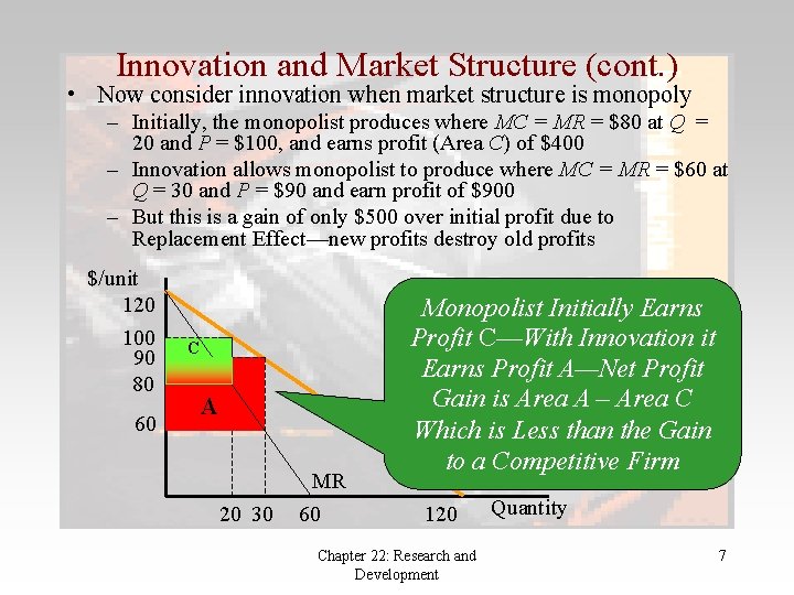
Innovation and Market Structure (cont. ) • Now consider innovation when market structure is monopoly – Initially, the monopolist produces where MC = MR = $80 at Q = 20 and P = $100, and earns profit (Area C) of $400 – Innovation allows monopolist to produce where MC = MR = $60 at Q = 30 and P = $90 and earn profit of $900 – But this is a gain of only $500 over initial profit due to Replacement Effect—new profits destroy old profits $/unit 120 100 90 80 60 C A 20 30 MR 60 Monopolist Initially Earns Profit C—With Innovation it Earns Profit A—Net Profit Gain is Area A – Area C Which is Less than the Gain Demand to a Competitive Firm 120 Chapter 22: Research and Development Quantity 7

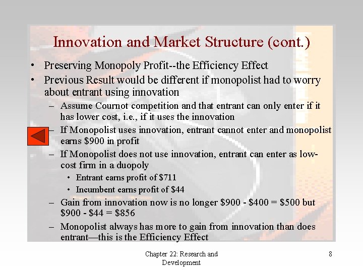
Innovation and Market Structure (cont. ) • Preserving Monopoly Profit--the Efficiency Effect • Previous Result would be different if monopolist had to worry about entrant using innovation – Assume Cournot competition and that entrant can only enter if it has lower cost, i. e. , if it uses the innovation – If Monopolist uses innovation, entrant cannot enter and monopolist earns $900 in profit – If Monopolist does not use innovation, entrant can enter as lowcost firm in a duopoly • Entrant earns profit of $711 • Incumbent earns profit of $44 – Gain from innovation now is no longer $900 - $400 = $500 but $900 - $44 = $856 – Monopolist always has more to gain from innovation than does entrant—this is the Efficiency Effect Chapter 22: Research and Development 8

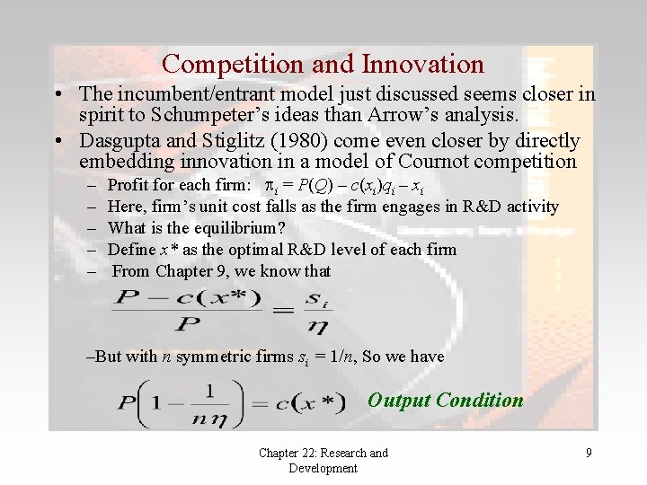
Competition and Innovation • The incumbent/entrant model just discussed seems closer in spirit to Schumpeter’s ideas than Arrow’s analysis. • Dasgupta and Stiglitz (1980) come even closer by directly embedding innovation in a model of Cournot competition – – – Profit for each firm: i = P(Q) – c(xi)qi – xi Here, firm’s unit cost falls as the firm engages in R&D activity What is the equilibrium? Define x* as the optimal R&D level of each firm From Chapter 9, we know that –But with n symmetric firms si = 1/n, So we have Output Condition Chapter 22: Research and Development 9

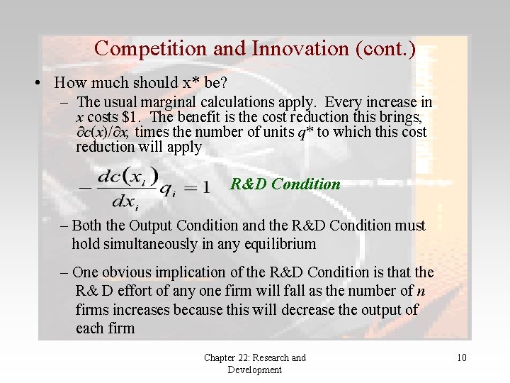
Competition and Innovation (cont. ) • How much should x* be? – The usual marginal calculations apply. Every increase in x costs $1. The benefit is the cost reduction this brings, c(x)/ x, times the number of units q* to which this cost reduction will apply R&D Condition – Both the Output Condition and the R&D Condition must hold simultaneously in any equilibrium – One obvious implication of the R&D Condition is that the R& D effort of any one firm will fall as the number of n firms increases because this will decrease the output of each firm Chapter 22: Research and Development 10

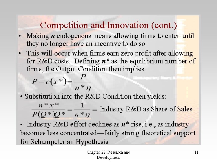
Competition and Innovation (cont. ) • Making n endogenous means allowing firms to enter until they no longer have an incentive to do so • This will occur when firms earn zero profit after allowing for R&D costs. Defining n* as the equilibrium number of firms, the Output Condition then implies: • Substitution into the R&D Condition then yields: Industry R&D as Share of Sales • Industry R&D effort declines as n* rise, i. e. , as industry becomes less concentrated—fairly strong theoretical support for Schumpeterian Hypothesis Chapter 22: Research and Development 11

Competition and Innovation (cont. ) • But empirical support for Schumpeterian view is mixed – Need to control for science-based sectors (e. g. , chemicals, pharmaceuticals, and electronics) and non-technology based sectors (e. g. , restaurants and hair stylists)—R&D much more likely in science-based sectors regardless of firm size – Need also to distinguish between R&D expenditures and true innovations. Common finding [e. g. , Cohen and Klepper (1996)], is that large firms do somewhat more R&D but achieve less real innovative breakthroughs—e. g. , Apple produced the first PC – Market structure is endogenous. Innovations might create industry giants (e. g. , Alcoa) not the other way around. • Bottom Line: Validity of Schumpeterian hypotheses is still undetermined Chapter 22: Research and Development 12

R&D Spillovers and Cooperative R&D • Technological break-throughs by one firm often “spill over’ to other firms – Spillover is unlikely to be complete but likely to arise to some extent – We can model this in the Dasgupta Stiglitz world by now writing a firm’s unit cost as a function of both its own and its rival’s R&D • c 1 = c – x 1 - x 2 • c 2 = c – x 2 - x 1 • To obtain solution, need also to assume that R&D is now subject to diminishing returns, i. e. , R&D cost is r(x) = x 2/2. • In this setting, response of firm 1’s R&D to firm 2’s R&D depends on size of spillover term . – When is small, R&D expenditures are strategic substitutes—the more firm 1 does the less firm 2 will do – When is large, R&D expenditures are strategic complements—the more firm 1 does the more firm 2 will do Chapter 22: Research and Development 13

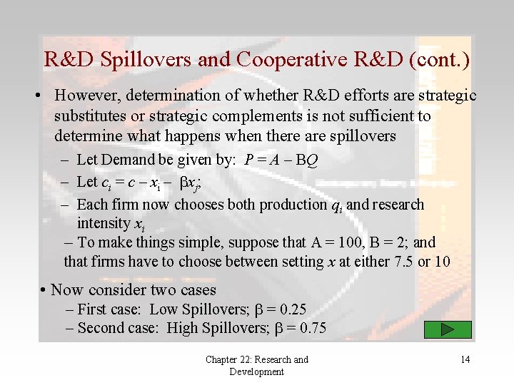
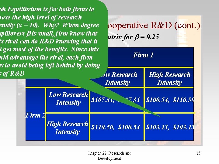
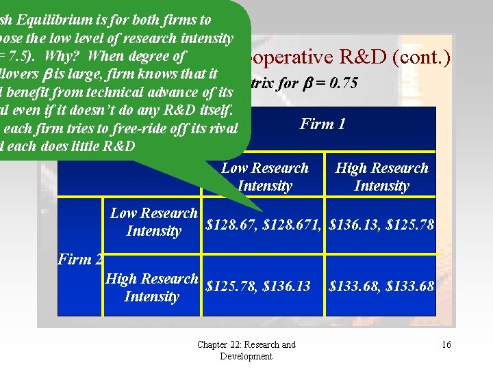
R&D Spillovers and Cooperative R&D (cont. ) • However, determination of whether R&D efforts are strategic substitutes or strategic complements is not sufficient to determine what happens when there are spillovers – Let Demand be given by: P = A – BQ – Let ci = c – xi – xj; – Each firm now chooses both production qi and research intensity xi – To make things simple, suppose that A = 100, B = 2; and that firms have to choose between setting x at either 7. 5 or 10 • Now consider two cases – First case: Low Spillovers; = 0. 25 – Second case: High Spillovers; = 0. 75 Chapter 22: Research and Development 14

sh Equilibrium is for both firms to oose the high level of research ensity (x. R&D = 10). Spillovers Why? When degree and Cooperative R&D (cont. ) spillovers is small, firm know that The Pay-Off Matrix for = 0. 25 ts rival can do R&D knowing that it l get most of the benefits. Since this Firm 1 uld advantage the rival, each firm es to avoid being left behind by doing s of R&D Low Research High Research Intensity Low Research $107. 31, $107. 31 $100. 54, $110. 50 Intensity Firm 2 High Research $110. 50, $100. 54 $103. 13, $103. 13 Intensity Chapter 22: Research and Development 15

sh Equilibrium is for both firms to oose the low level of research intensity = 7. 5). R&D Why? When degree of and Cooperative R&D (cont. ) Spillovers is large, firm knows that it The Pay-Off Matrix for = 0. 75 l benefit from technical advance of its al even if it doesn’t do any R&D itself. Firm 1 each firm tries to free-ride off its rival d each does little R&D Low Research High Research Intensity Low Research $128. 67, $128. 671, $136. 13, $125. 78 Intensity Firm 2 High Research $125. 78, $136. 13 Intensity Chapter 22: Research and Development $133. 68, $133. 68 16

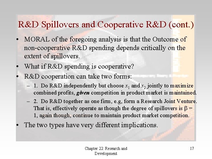
R&D Spillovers and Cooperative R&D (cont. ) • MORAL of the foregoing analysis is that the Outcome of non-cooperative R&D spending depends critically on the extent of spillovers. • What if R&D spending is cooperative? • R&D cooperation can take two forms: – 1. Do R&D independently but choose x 1 and x 2 jointly to maximize combined profits, given competition in product market is maintained. – 2. Do R&D together as one firm, e. g, form a Research Joint Venture. That is, effectively operate as though the degree of spillovers is = 1, again though, continue to maintain product market competition. • The two types have very different implications. Chapter 22: Research and Development 17

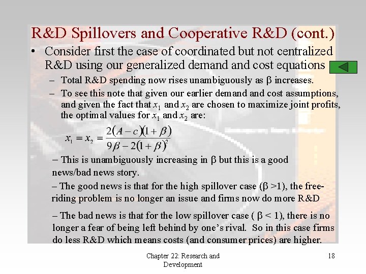
R&D Spillovers and Cooperative R&D (cont. ) • Consider first the case of coordinated but not centralized R&D using our generalized demand cost equations – Total R&D spending now rises unambiguously as increases. – To see this note that given our earlier demand cost assumptions, and given the fact that x 1 and x 2 are chosen to maximize joint profits, the optimal values for x 1 and x 2 are: – This is unambiguously increasing in but this is a good news/bad news story. – The good news is that for the high spillover case ( >1), the freeriding problem is no longer an issue and firms now do more R&D – The bad news is that for the low spillover case ( < 1), there is no longer a fear of being left behind by one’s rival. So in this case firms do less R&D which means costs (and consumer prices) are higher. Chapter 22: Research and Development 18

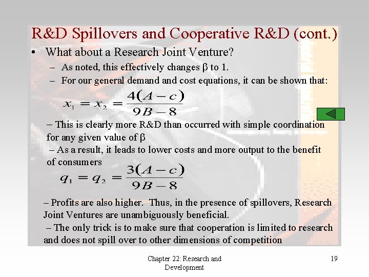
R&D Spillovers and Cooperative R&D (cont. ) • What about a Research Joint Venture? – As noted, this effectively changes to 1. – For our general demand cost equations, it can be shown that: – This is clearly more R&D than occurred with simple coordination for any given value of – As a result, it leads to lower costs and more output to the benefit of consumers – Profits are also higher. Thus, in the presence of spillovers, Research Joint Ventures are unambiguously beneficial. – The only trick is to make sure that cooperation is limited to research and does not spill over to other dimensions of competition Chapter 22: Research and Development 19