Particle Swarm Optimization Using the HP Prime Presented

Particle Swarm Optimization Using the HP Prime Presented by Namir Shammas 1

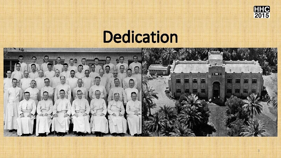
Dedication I dedicate this tutorial, with an immense sense of gratitude and thankfulness, to the fine Boston College Jesuits who spent decades working in Iraq to educate students in Baghdad College and Al-Hikmat University. They instilled in us the power to be self-taught! No words can fully thank them for that gift alone. 2

Dedication 3

Particle Swarm Optimization • Efficient method for stochastic optimization. • Is based on the movement and cleverness of swarms in the search space to locate the best solution. • Was developed by James Kennedy in 1995. • Algorithm simulates the use of particles (agents) making up a swarm moving throughout the search space looking for the best solution. 4

Particle Swarm Optimization • Every particle represents a point flying in a multidimensional space. • Each particle adjusts its flying metrics influenced by its own experience and in addition by the experience of other particles. • Each particle keeps track of it’s personal best (lowest/highest function value), part. Best(i). • The particles keeps track of the global best, glob. Best. 3

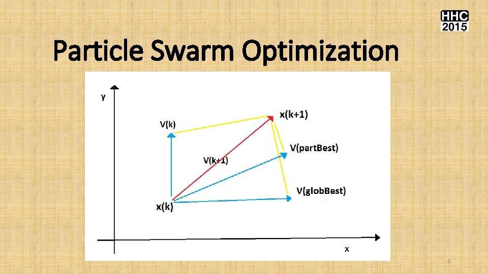
Particle Swarm Optimization 6

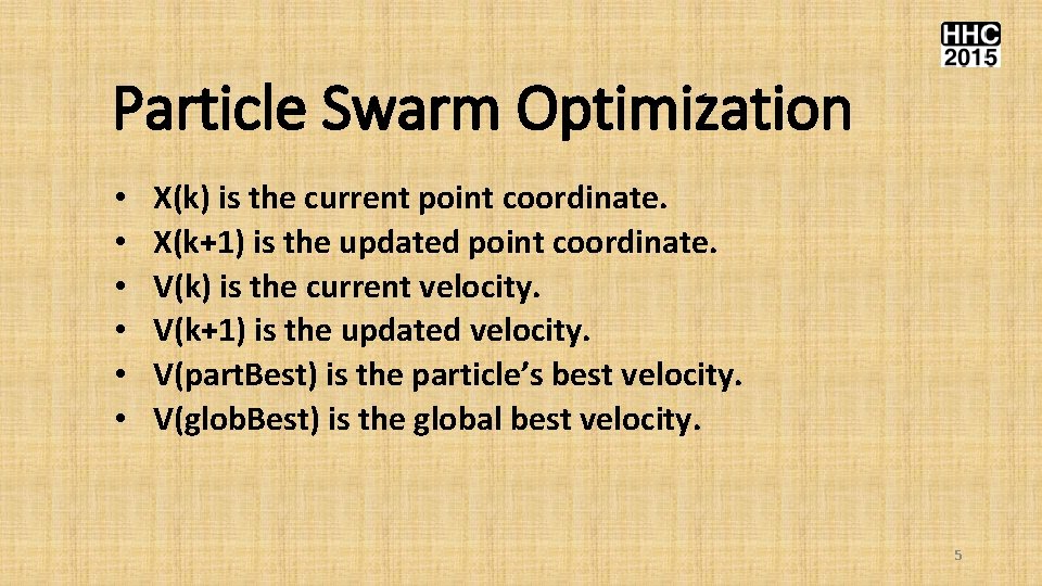
Particle Swarm Optimization • • • X(k) is the current point coordinate. X(k+1) is the updated point coordinate. V(k) is the current velocity. V(k+1) is the updated velocity. V(part. Best) is the particle’s best velocity. V(glob. Best) is the global best velocity. 5

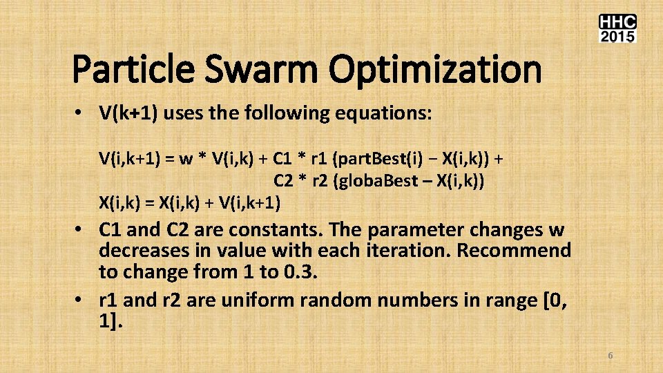
Particle Swarm Optimization • V(k+1) uses the following equations: V(i, k+1) = w * V(i, k) + C 1 * r 1 (part. Best(i) − X(i, k)) + C 2 * r 2 (globa. Best – X(i, k)) X(i, k) = X(i, k) + V(i, k+1) • C 1 and C 2 are constants. The parameter changes w decreases in value with each iteration. Recommend to change from 1 to 0. 3. • r 1 and r 2 are uniform random numbers in range [0, 1]. 6

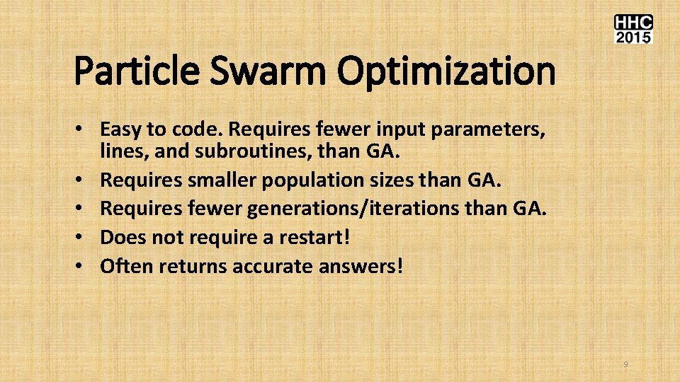
Particle Swarm Optimization • Easy to code. Requires fewer input parameters, lines, and subroutines, than GA. • Requires smaller population sizes than GA. • Requires fewer generations/iterations than GA. • Does not require a restart! • Often returns accurate answers! 9

HP Prime Implementation • Function PSO returns the best solution for optimized function My. Fx. • Parameters for PSO are: • • Number of variables. Population size (number of probes). Maximum generations (i. e. iterations). Two arrays that define the lower and upper bounds for each variable. 8

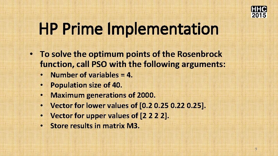
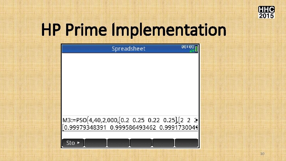
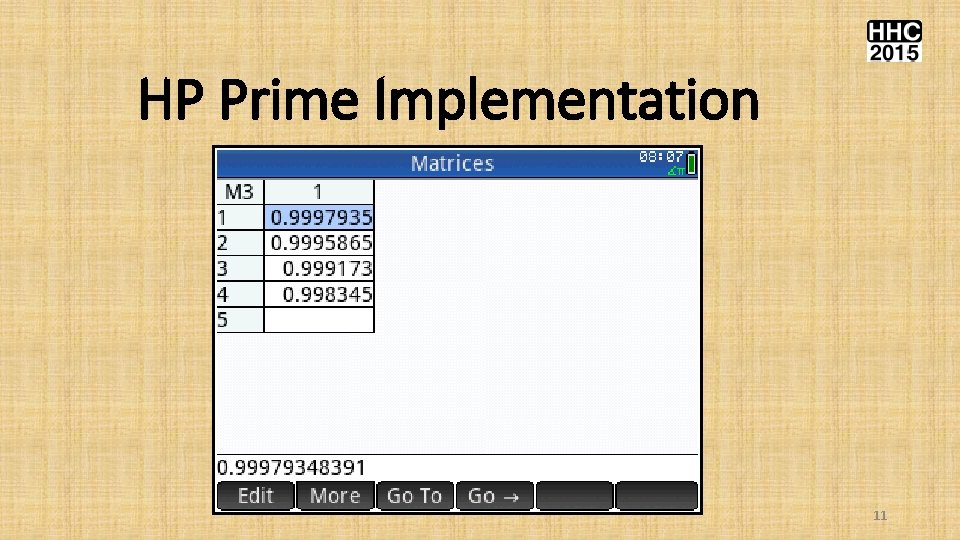
HP Prime Implementation • To solve the optimum points of the Rosenbrock function, call PSO with the following arguments: • • • Number of variables = 4. Population size of 40. Maximum generations of 2000. Vector for lower values of [0. 25 0. 22 0. 25]. Vector for upper values of [2 2 2 2]. Store results in matrix M 3. 9

HP Prime Implementation 10

HP Prime Implementation 11

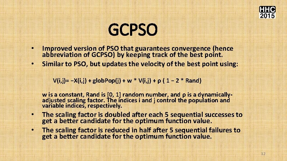
GCPSO • • Improved version of PSO that guarantees convergence (hence abbreviation of GCPSO) by keeping track of the best point. Similar to PSO, but updates the velocity of the best point using: V(i, j)= −X(i, j) + glob. Pop(j) + w * V(i, j) + ρ ( 1 − 2 * Rand) w is a constant, Rand is [0, 1] random number, and ρ is a dynamicallyadjusted scaling factor. The indices i and j control the population and variable indices, respectively. • • The scaling factor is doubled after each 5 sequential successes to get a better candidate for the optimum function value. The scaling factor is reduced in half after 5 sequential failures to get a better candidate for the optimum function value. 12

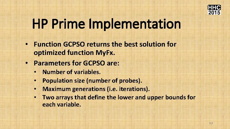
HP Prime Implementation • Function GCPSO returns the best solution for optimized function My. Fx. • Parameters for GCPSO are: • • Number of variables. Population size (number of probes). Maximum generations (i. e. iterations). Two arrays that define the lower and upper bounds for each variable. 13

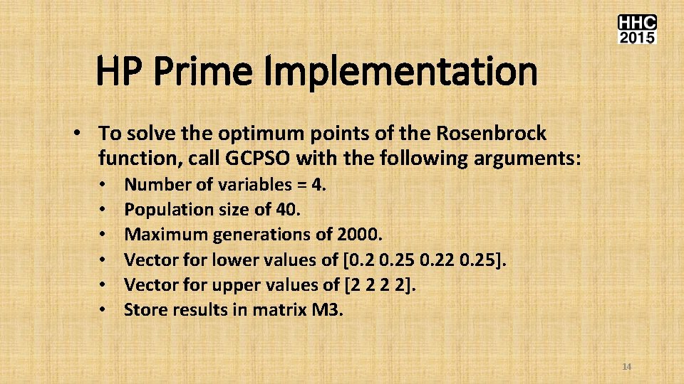
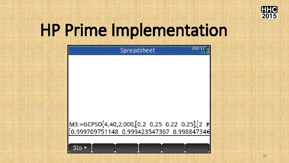
HP Prime Implementation • To solve the optimum points of the Rosenbrock function, call GCPSO with the following arguments: • • • Number of variables = 4. Population size of 40. Maximum generations of 2000. Vector for lower values of [0. 25 0. 22 0. 25]. Vector for upper values of [2 2 2 2]. Store results in matrix M 3. 14

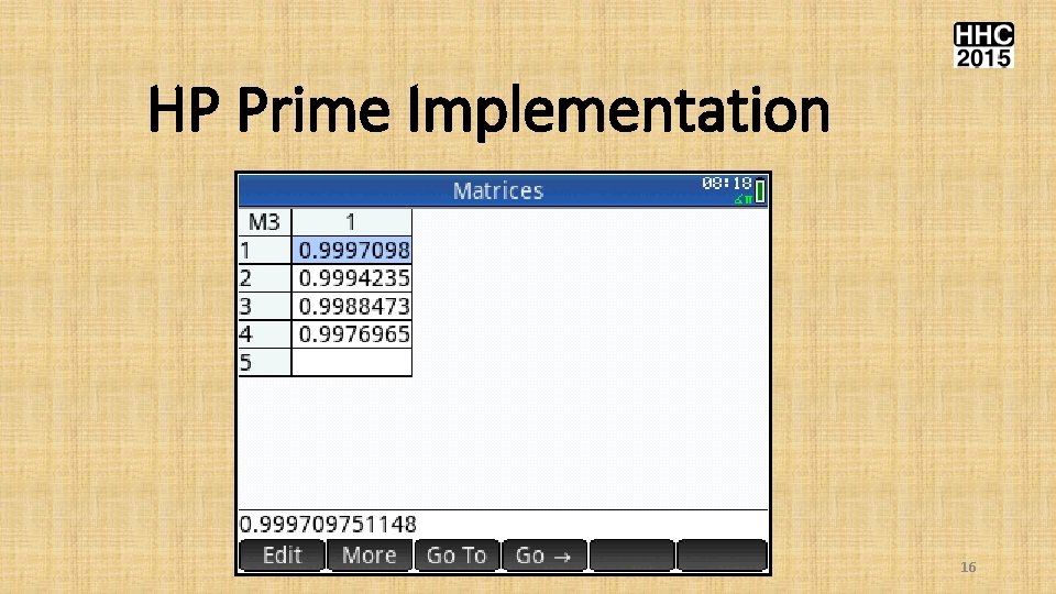
HP Prime Implementation 15

HP Prime Implementation 16

BONUS MATERIAL! 17

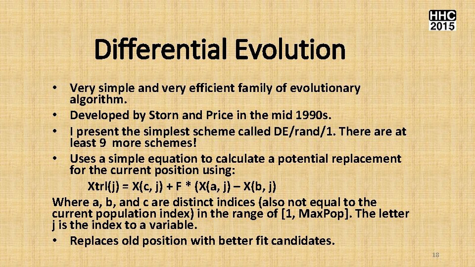
Differential Evolution • Very simple and very efficient family of evolutionary algorithm. • Developed by Storn and Price in the mid 1990 s. • I present the simplest scheme called DE/rand/1. There at least 9 more schemes! • Uses a simple equation to calculate a potential replacement for the current position using: Xtrl(j) = X(c, j) + F * (X(a, j) – X(b, j) Where a, b, and c are distinct indices (also not equal to the current population index) in the range of [1, Max. Pop]. The letter j is the index to a variable. • Replaces old position with better fit candidates. 18

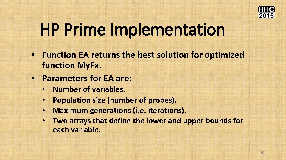
HP Prime Implementation • Function EA returns the best solution for optimized function My. Fx. • Parameters for EA are: • • Number of variables. Population size (number of probes). Maximum generations (i. e. iterations). Two arrays that define the lower and upper bounds for each variable. 19

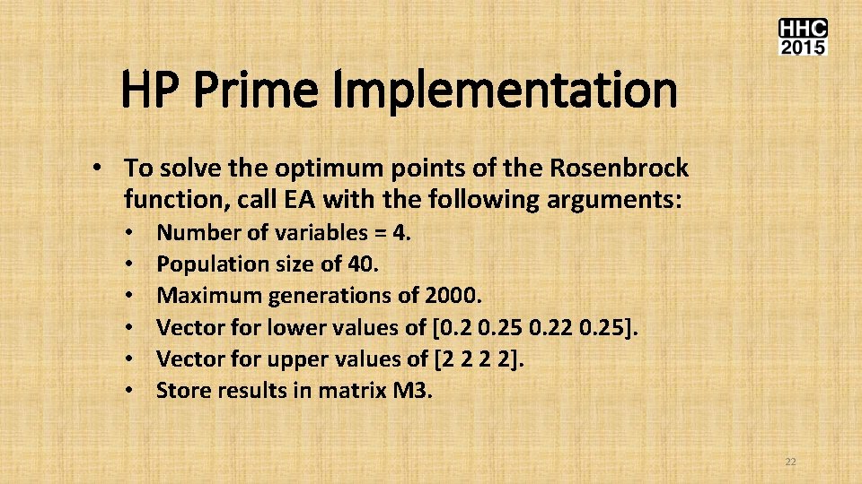
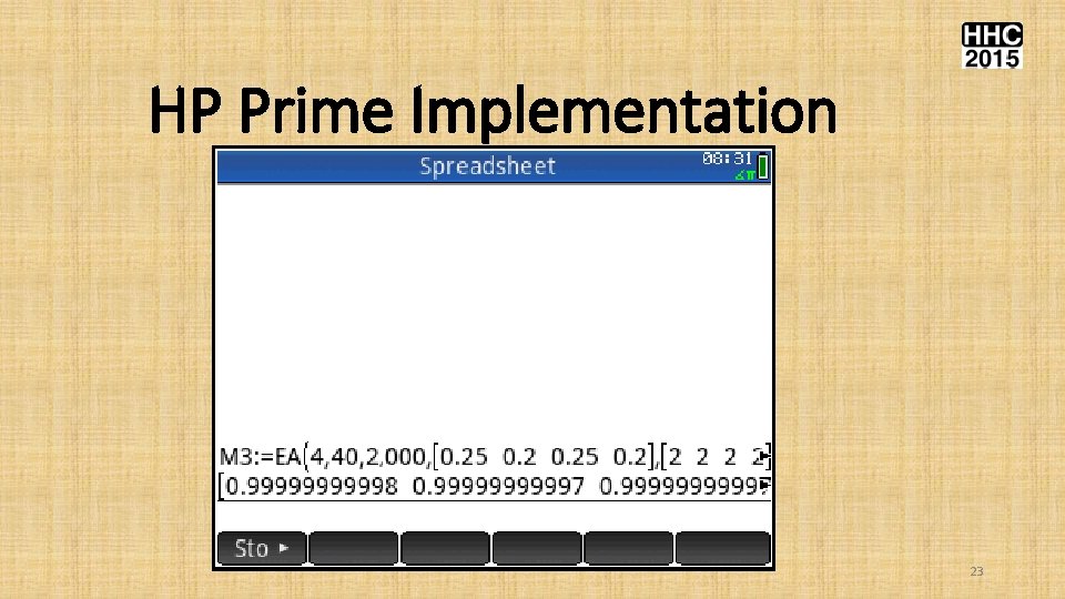
HP Prime Implementation • To solve the optimum points of the Rosenbrock function, call EA with the following arguments: • • • Number of variables = 4. Population size of 40. Maximum generations of 2000. Vector for lower values of [0. 25 0. 22 0. 25]. Vector for upper values of [2 2 2 2]. Store results in matrix M 3. 22

HP Prime Implementation 23

HP Prime Implementation 22

HP Prime Implementation Paraphrasing actor Steve Buscemi in Escape from LA, This crowd loves a winner! 22

Final Remarks • Evolutionary algorithms for optimization are a mix between science, experimentation, and art. • There is a large number of variants for the various evolutionary algorithms. Number exceeds by far the number of classical optimization methods and their variants. • Complexity of algorithm does not always equal superiority of performance. Some cleverly designed simple algorithm can perform very well. 23

No Free Lunch in Search and Optimization • There is no single algorithm that can solve all optimization problems! Principle is abbreviated as NFL. • Concept proposed by Wolpert and Macready in 1997. • You will need to experiment with several algorithms to find the best one for your problem. • Given an algorithm A, researchers have found that A may succeed with p % of the problems, while some other algorithms, collectively call them B, will solve (100 -p)% of the remaining problems. B may represent one of more algorithms. 24

No Free Lunch in Search and Optimization (cont. ) • See the following web sites: • • https: //en. wikipedia. org/wiki/No_free_lunch_in_search_and_optim ization http: //www. no-free-lunch. org/ www. santafe. edu/media/workingpapers/12 -10 -017. pdf www. no-free-lunch. org/Wo. Ma 96 a. pdf 28

References • • • Clever Algorithms-Nature-Inspired Programming Recipes, first ed. , 2011, by Jason Brownlee. (Available for online reading). Handbook of Metaheuristics, first ed. , 2003, by Fred Glover and Gary A. Kochenberger. Particle Swarm Optimization, first ed. , 2006, by Maurice Clerc. Practical Genetic Algorithms, second ed. , 2004, by Randy L. Haupt and Sue Ellen Haupt. Evolutionary Optimization Algorithms, first ed. , 2015, by Dan Simon. 29

Thank You!! 30