Paper G Gyarmati I Szunyogh and D J

Paper G. Gyarmati, I. Szunyogh, and D. J. Patil, 2003: Local predictability in a simple model of atmospheric balance, Nonlinear Processes in Geophysics 10: 183 -196 http: //www. copernicus. org/EGU/npg/10/183. htm

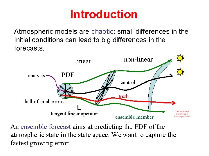
Introduction Atmospheric models are chaotic: small differences in the initial conditions can lead to big differences in the forecasts. linear analysis non-linear PDF control ball of small errors truth L tangent linear operator ensemble member An ensemble forecast aims at predicting the PDF of the atmospheric state in the state space. We want to capture the fastest growing error.

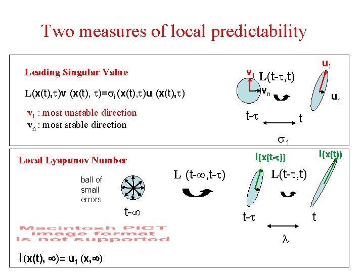
Two measures of local predictability v 1 Leading Singular Value t 1 L(t- , t) t- t l l (x(t), ) u 1 (x, ) l(x(t)) l(x(t- )) L (t- , t- ) t- un t- Local Lyapunov Number ball of small errors L(t- , t) vn L(x(t), )vi (x(t), )= i (x(t), )ui (x(t), ) v 1 : most unstable direction vn : most stable direction u 1

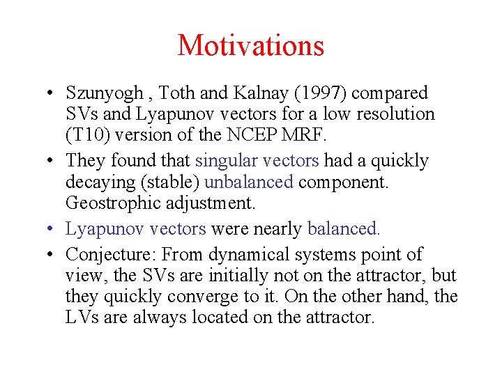
Motivations • Szunyogh , Toth and Kalnay (1997) compared SVs and Lyapunov vectors for a low resolution (T 10) version of the NCEP MRF. • They found that singular vectors had a quickly decaying (stable) unbalanced component. Geostrophic adjustment. • Lyapunov vectors were nearly balanced. • Conjecture: From dynamical systems point of view, the SVs are initially not on the attractor, but they quickly converge to it. On the other hand, the LVs are always located on the attractor.

Motivations II. • Lorenz (1986) derived the L 5 model to prove the existence of the slow manifold. • L 5 is the highest truncated version of the shallow water equations. • Existence of the slow manifold for the L 5 model had not been proved for the nondissipative case for 10 years. • Bokhove and Sheperd (1996) finally showed that the slow manifold can exist in the nondissipative case.

Main Goal • To demonstrate, that the characteristic difference between the SVs and LVs in terms of balance is due to the existence of multiple time scales (the existence of an attractor, i. e dissipative forces, is not a necessary condition. ) • We choose a simple chaotic model that maintains two distinct time scales, but which is nondissipative (i. e has no attractor).

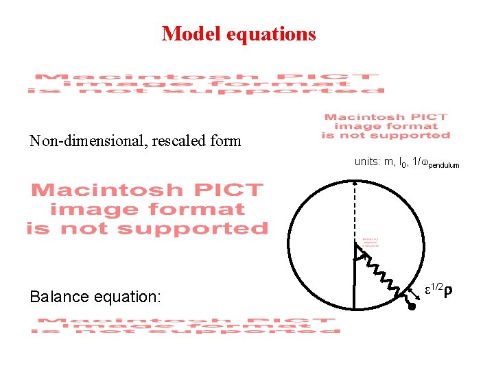
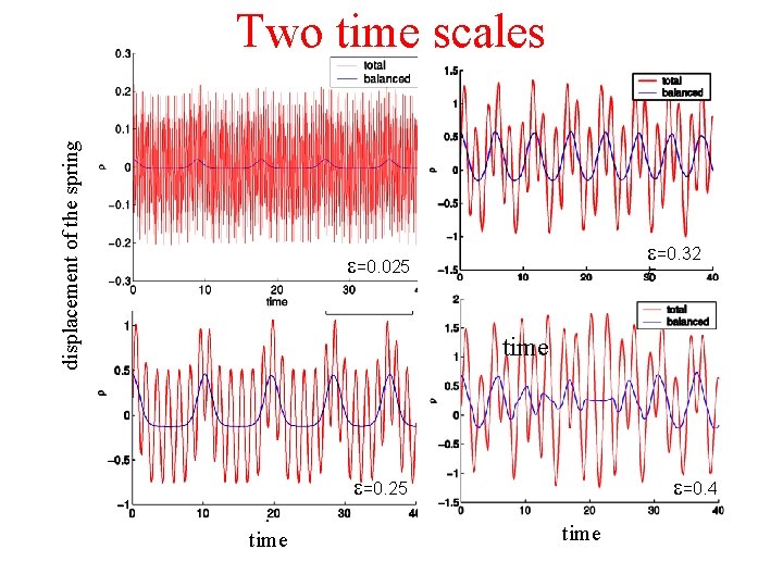
The model • Camassa (1995): the L 5 is a nonlinearly coupled system of a nonlinear pendulum and a linear oscillator (spring). There are only 4 independent dynamical variables. • Lynch (1996, 2002): A slight modification of the coupling term in L 5 leads to the swinging spring model. It has two time scales, but no attractor.

Model equations Non-dimensional, rescaled form units: m, l 0, 1/ pendulum Balance equation: 1/2

displacement of the spring Two time scales =0. 32 =0. 025 5 time =0. 25 time =0. 4 time

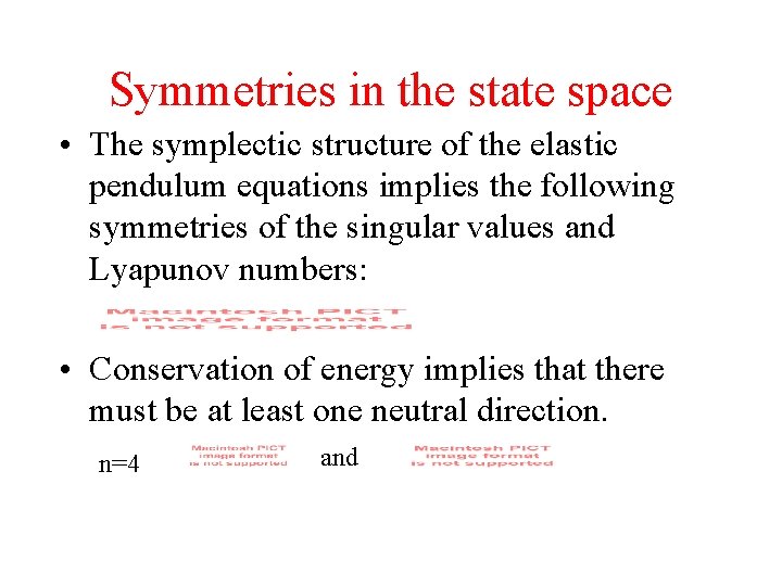
Symmetries in the state space • The symplectic structure of the elastic pendulum equations implies the following symmetries of the singular values and Lyapunov numbers: • Conservation of energy implies that there must be at least one neutral direction. n=4 and

Numerical Solutions • The system can not be solved analytically. • We need to solve with a numerical method. • A high order symplectic integrator is needed, because • we want to preserve the symmetry of the singular values • structure preserving schemes are know to be more efficient in preserving energy, than energy preserving schemes in conserving the structure • For a non-separable Hamiltonian system structure preserving integrators are symmetric composition schemes. • We created a family of symplectic integrators for the elastic pendulum based on Mc. Lachlan’s (1995) generalized theory.

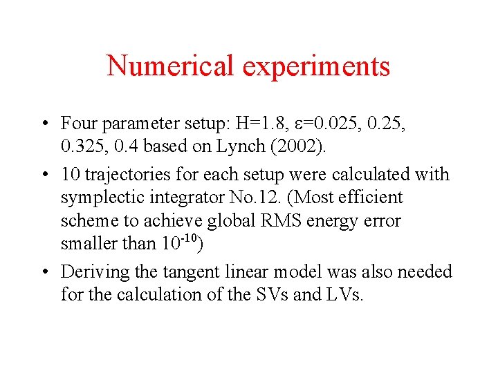
Numerical experiments • Four parameter setup: H=1. 8, =0. 025, 0. 325, 0. 4 based on Lynch (2002). • 10 trajectories for each setup were calculated with symplectic integrator No. 12. (Most efficient scheme to achieve global RMS energy error smaller than 10 -10) • Deriving the tangent linear model was also needed for the calculation of the SVs and LVs.

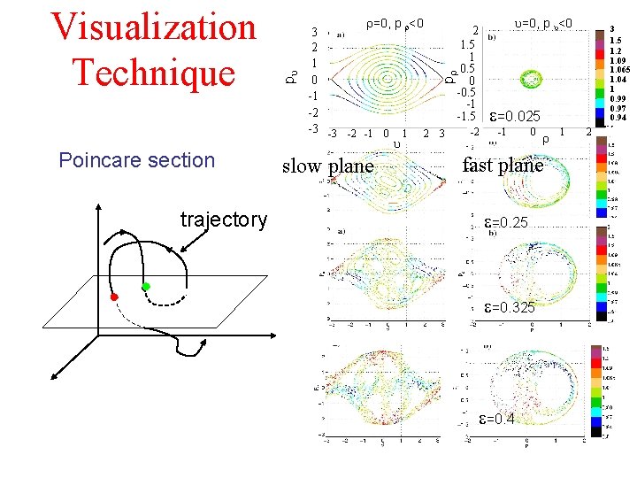
Poincare section trajectory =0, p <0 2 3 1. 5 2 1 1 0. 5 0 0 -0. 5 -1 -1 -2 -1. 5 -3 -3 -2 -1 0 1 2 3 -2 slow plane =0, p <0 3 1. 5 1. 2 1. 09 1. 065 1. 04 1 0. 99 0. 97 0. 94 p p Visualization Technique =0. 025 -1 0 fast plane =0. 25 =0. 325 =0. 4 1 2

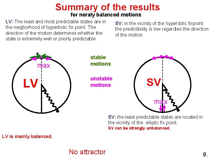
Summary of the results for neraly balanced motions LV: The least and most predictable states are in the neigborhood of hyperbolic fix point. The direction of the motion determines whether the state is extremely well or poorly predictable. max LV SV: in the vicinity of the hyperdolic fixpoint the predictibility is low regardles the direction of the motion. stable motions unstable motions SV max SV: the least predictable states are located in the vicinity of the elliptic fix point. SV can be strongly unbalanced. LV is mainly balanced. No attractor 9.

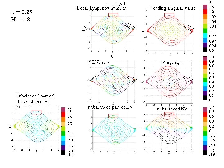
=0, p <0 Local Lyapunov number = 0. 25 leading singular value p H = 1. 8 < LV, v 4 > Unbalanced part of the displacement 1. 5 0. 9 0. 6 0. 3 0. 2 0 -0. 1 -0. 3 -0. 5 -0. 8 -1. 6 unbalanced part of LV < u 4 , v 4 > unbalanced SV 3 1. 5 1. 2 1. 09 1. 065 1. 04 1 0. 99 0. 97 0. 94 0. 5 1. 0 0. 9 0. 8 0. 7 0. 6 0. 5 0. 4 0. 3 0. 2 0. 1 0 1. 7 0. 9 0. 6 0. 3 0. 2 0 -0. 1 -0. 3 -0. 5 -0. 8 -1. 6

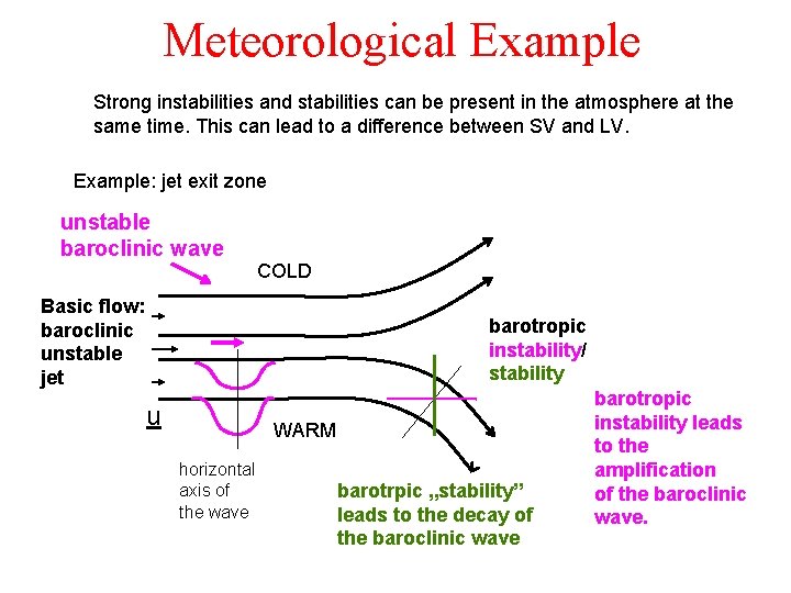
Meteorological Example Strong instabilities and stabilities can be present in the atmosphere at the same time. This can lead to a difference between SV and LV. Example: jet exit zone unstable baroclinic wave COLD Basic flow: baroclinic unstable jet barotropic instability/ stability u WARM horizontal axis of the wave barotrpic „stability” leads to the decay of the baroclinic wave barotropic instability leads to the amplification of the baroclinic wave.

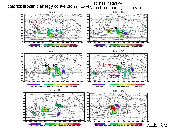
isolines: negative colors: baroclinic energy conversion (J*day/kg)barotropic energy conversion baroclinic -400 - -600 barotropi c -400 - -1600 baroclinic Mike Oz

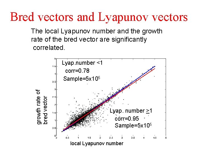
Bred vectors and Lyapunov vectors The local Lyapunov number and the growth rate of the bred vector are significantly correlated. growth rate of bred vector Lyap. number <1 corr=0. 78 Sample=5 x 105 Lyap. number >1 corr=0. 95 Sample=5 x 105 local Lyapunov number

Conclusions • When the atmospheric state is nearly balanced, the SVs can have a strongly unbalanced component, while the LVs are also nearly balanced. This seems to be fundamental property of systems with more time scales, which exists independently of the dissipative or non-dissipative nature of the system. • There are cases when the Lyapunov number indicates extremely high predictability, while the leading singular value indicates extremely low predictability. Barotropic instability is a process that can lead to similar behavior in the atmosphere. (We are planning to carry out more research in this area. )