OLAP and Data Warehousing Slides courtesy of Julia

OLAP and Data Warehousing Slides courtesy of: Julia Stoyanovitch Columbia University Surajit Chaudhuri Microsoft Research, Redmond, WA, USA surajitc@microsoft. com Umeshwar Dayal Hewlett-Packard Labs. , Palo Alto, CA, USA dayal@hpl. hp. com 1

What is OLAP? u On-Line Analytical Processing u Information technology to help the knowledge worker (executive, manager, analyst) make faster and better decisions. u OLAP is an element of decision support systems (DSS). © Surajit Chaudhuri, Umeshwar Dayal 23

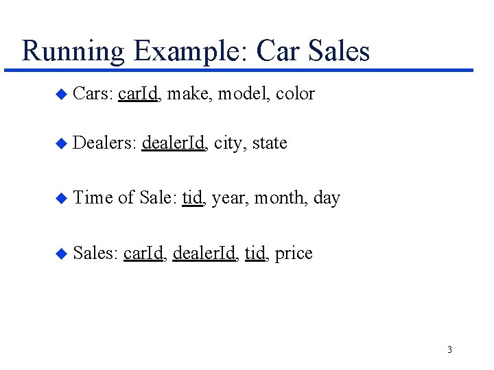
Running Example: Car Sales u Cars: car. Id, make, model, color u Dealers: u Time dealer. Id, city, state of Sale: tid, year, month, day u Sales: car. Id, dealer. Id, tid, price 3

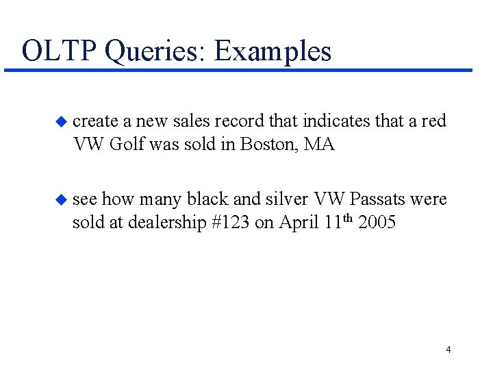
OLTP Queries: Examples u create a new sales record that indicates that a red VW Golf was sold in Boston, MA u see how many black and silver VW Passats were sold at dealership #123 on April 11 th 2005 4

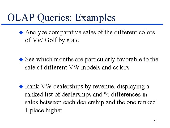
OLAP Queries: Examples u Analyze comparative sales of the different colors of VW Golf by state u See which months are particularly favorable to the sale of different VW models and colors u Rank VW dealerships by revenue, displaying a ranked list of dealerships and % differences in sales between each dealership and the one ranked 1 place higher 5

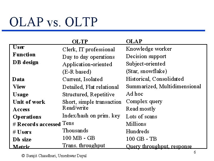
OLAP vs. OLTP User Clerk, IT professional Function Day to day operations DB design Application-oriented (E-R based) Data Current, Isolated View Detailed, Flat relational Usage Structured, Repetitive Unit of work Short, simple transaction Read/write Access Index/hash on prim. key Operations # Records accessed Tens Thousands # Users 100 MB - GB Db size Trans. throughput Metric © Surajit Chaudhuri, Umeshwar Dayal OLAP Knowledge worker Decision support Subject-oriented (Star, snowflake) Historical, Consolidated Summarized, Multidimensional Ad hoc Complex query Read mostly Lots of scans Millions Hundreds 100 GB - TB Query throughput, response 6

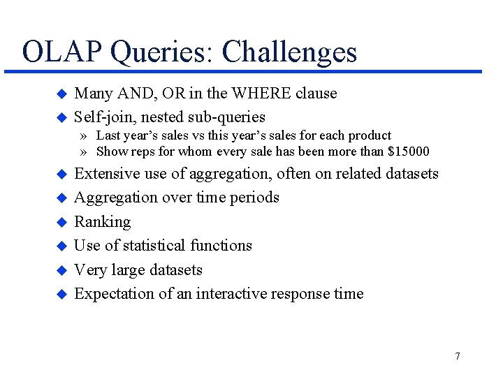
OLAP Queries: Challenges u u Many AND, OR in the WHERE clause Self-join, nested sub-queries » Last year’s sales vs this year’s sales for each product » Show reps for whom every sale has been more than $15000 u u u Extensive use of aggregation, often on related datasets Aggregation over time periods Ranking Use of statistical functions Very large datasets Expectation of an interactive response time 7

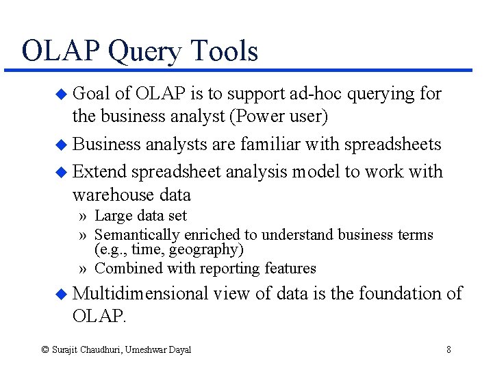
OLAP Query Tools u Goal of OLAP is to support ad-hoc querying for the business analyst (Power user) u Business analysts are familiar with spreadsheets u Extend spreadsheet analysis model to work with warehouse data » Large data set » Semantically enriched to understand business terms (e. g. , time, geography) » Combined with reporting features u Multidimensional view of data is the foundation of OLAP. © Surajit Chaudhuri, Umeshwar Dayal 8

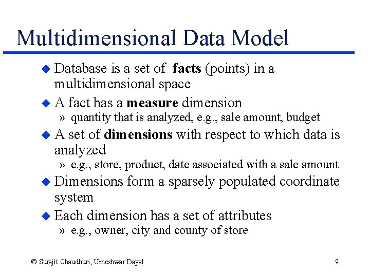
Multidimensional Data Model u Database is a set of facts (points) in a multidimensional space u A fact has a measure dimension » quantity that is analyzed, e. g. , sale amount, budget u. A set of dimensions with respect to which data is analyzed » e. g. , store, product, date associated with a sale amount u Dimensions form a sparsely populated coordinate system u Each dimension has a set of attributes » e. g. , owner, city and county of store © Surajit Chaudhuri, Umeshwar Dayal 9

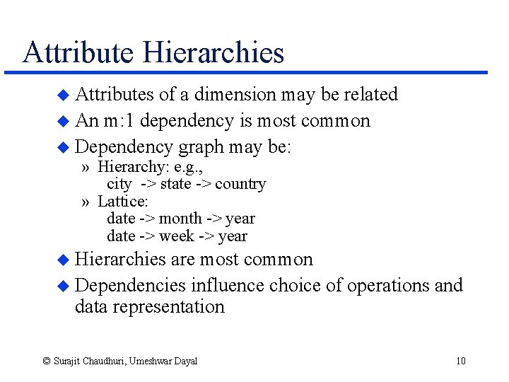
Attribute Hierarchies u Attributes of a dimension may be related u An m: 1 dependency is most common u Dependency graph may be: » Hierarchy: e. g. , city -> state -> country » Lattice: date -> month -> year date -> week -> year u Hierarchies are most common u Dependencies influence choice of operations and data representation © Surajit Chaudhuri, Umeshwar Dayal 10

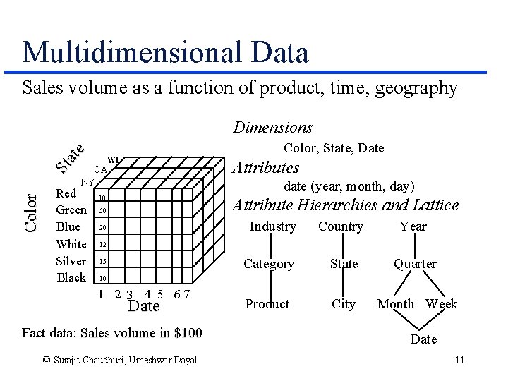
Multidimensional Data Sales volume as a function of product, time, geography St ate Dimensions Color, State, Date WI Attributes Color CA NY Red Green Blue White Silver Black date (year, month, day) 10 Attribute Hierarchies and Lattice 50 20 Industry Country Year Category State Quarter Product City Month Week 12 15 10 1 2 3 4 5 67 Date Fact data: Sales volume in $100 © Surajit Chaudhuri, Umeshwar Dayal Date 11

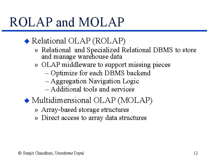
ROLAP and MOLAP u Relational OLAP (ROLAP) » Relational and Specialized Relational DBMS to store and manage warehouse data » OLAP middleware to support missing pieces – Optimize for each DBMS backend – Aggregation Navigation Logic – Additional tools and services u Multidimensional OLAP (MOLAP) » Array-based storage structures » Direct access to array data structures © Surajit Chaudhuri, Umeshwar Dayal 12

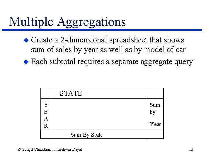
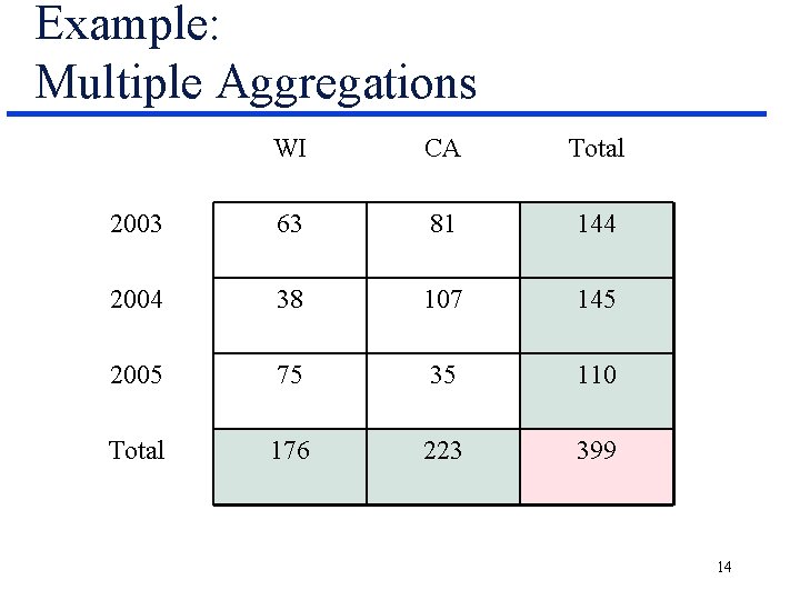
Multiple Aggregations u Create a 2 -dimensional spreadsheet that shows sum of sales by year as well as by model of car u Each subtotal requires a separate aggregate query STATE Y E A R Sum by Year Sum By State © Surajit Chaudhuri, Umeshwar Dayal 13

Example: Multiple Aggregations WI CA Total 2003 63 81 144 2004 38 107 145 2005 75 35 110 Total 176 223 399 14

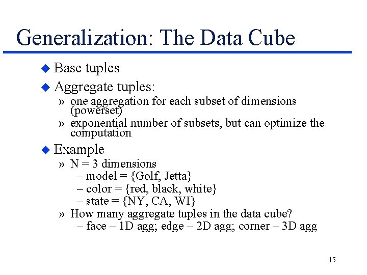
Generalization: The Data Cube u Base tuples u Aggregate tuples: » one aggregation for each subset of dimensions (powerset) » exponential number of subsets, but can optimize the computation u Example » N = 3 dimensions – model = {Golf, Jetta} – color = {red, black, white} – state = {NY, CA, WI} » How many aggregate tuples in the data cube? – face – 1 D agg; edge – 2 D agg; corner – 3 D agg 15

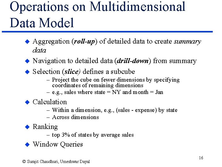
Operations on Multidimensional Data Model u u u Aggregation (roll-up) of detailed data to create summary data Navigation to detailed data (drill-down) from summary Selection (slice) defines a subcube – Project the cube on fewer dimensions by specifying coordinates of remaining dimensions – e. g. , sales where state = NY and month = Jan u Calculation – Within a dimension, e. g. , (sales - expense) by state – Across dimensions u Ranking – top 3% of states by average sales u Window Queries © Surajit Chaudhuri, Umeshwar Dayal 16

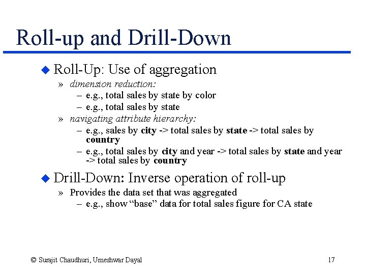
Roll-up and Drill-Down u Roll-Up: Use of aggregation » dimension reduction: – e. g. , total sales by state by color – e. g. , total sales by state » navigating attribute hierarchy: – e. g. , sales by city -> total sales by state -> total sales by country – e. g. , total sales by city and year -> total sales by state and year -> total sales by country u Drill-Down: Inverse operation of roll-up » Provides the data set that was aggregated – e. g. , show “base” data for total sales figure for CA state © Surajit Chaudhuri, Umeshwar Dayal 17

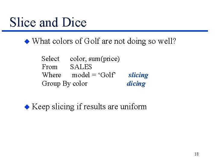
Slice and Dice u What colors of Golf are not doing so well? Select color, sum(price) From SALES Where model = ‘Golf’ slicing Group By color dicing u Keep slicing if results are uniform 18

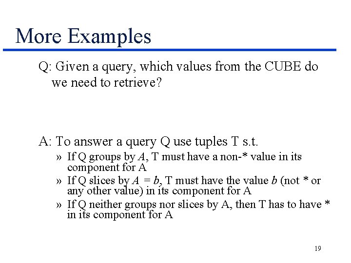
More Examples Q: Given a query, which values from the CUBE do we need to retrieve? A: To answer a query Q use tuples T s. t. » If Q groups by A, T must have a non-* value in its component for A » If Q slices by A = b, T must have the value b (not * or any other value) in its component for A » If Q neither groups nor slices by A, then T has to have * in its component for A 19

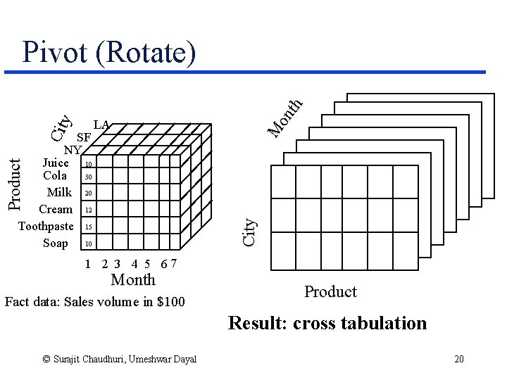
LA City Product SF NY Juice 10 Cola 50 Milk 20 Cream 12 Toothpaste 15 Soap 10 M on th Cit y Pivot (Rotate) 1 2 3 4 5 67 Month Fact data: Sales volume in $100 Product Result: cross tabulation © Surajit Chaudhuri, Umeshwar Dayal 20

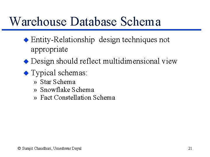
Warehouse Database Schema u Entity-Relationship design techniques not appropriate u Design should reflect multidimensional view u Typical schemas: » Star Schema » Snowflake Schema » Fact Constellation Schema © Surajit Chaudhuri, Umeshwar Dayal 21

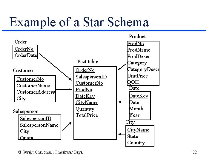
Example of a Star Schema Order. No Order. Date Fact table Customer. No Customer. Name Customer. Address City Salesperson. ID Salesperson. Name City Quota Order. No Salesperson. ID Customer. No Prod. No Date. Key City. Name Quantity Total. Price © Surajit Chaudhuri, Umeshwar Dayal Product Prod. No Prod. Name Prod. Descr Category. Descr Unit. Price QOH Date. Key Date Month Year City. Name State Country 22

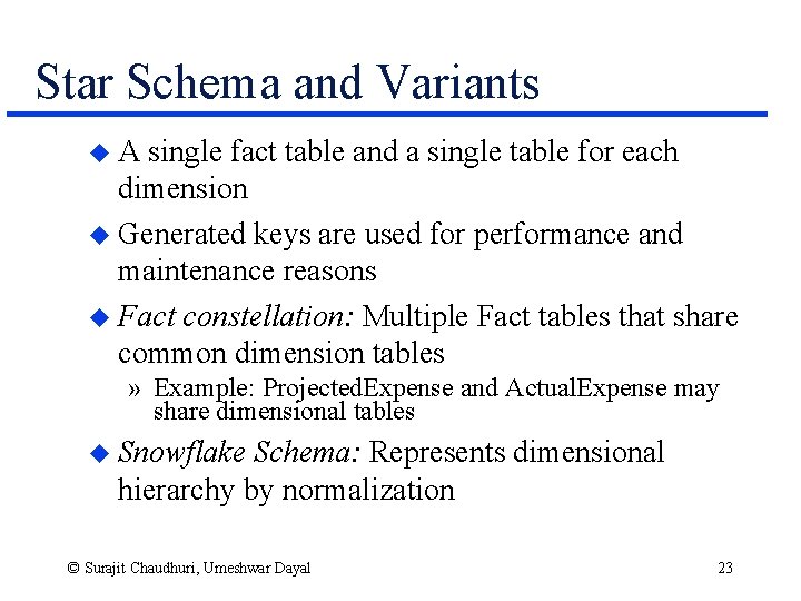
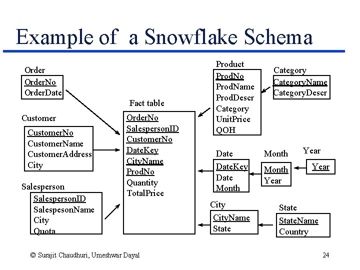
Star Schema and Variants u. A single fact table and a single table for each dimension u Generated keys are used for performance and maintenance reasons u Fact constellation: Multiple Fact tables that share common dimension tables » Example: Projected. Expense and Actual. Expense may share dimensional tables u Snowflake Schema: Represents dimensional hierarchy by normalization © Surajit Chaudhuri, Umeshwar Dayal 23

Example of a Snowflake Schema Order. No Order. Date Fact table Customer. No Customer. Name Customer. Address City Salesperson. ID Salespeson. Name City Quota Order. No Salesperson. ID Customer. No Date. Key City. Name Prod. No Quantity Total. Price © Surajit Chaudhuri, Umeshwar Dayal Product Prod. No Prod. Name Prod. Descr Category Unit. Price QOH Date. Key Date Month City. Name State Category. Name Category. Descr Month Year State. Name Country 24

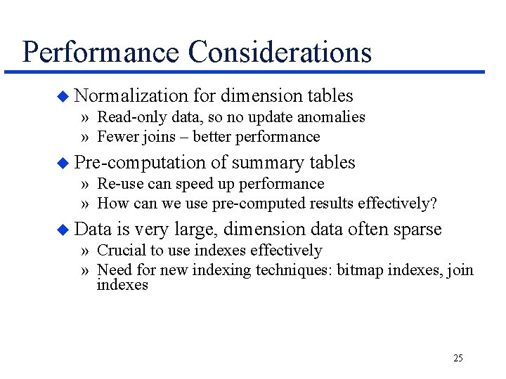
Performance Considerations u Normalization for dimension tables » Read-only data, so no update anomalies » Fewer joins – better performance u Pre-computation of summary tables » Re-use can speed up performance » How can we use pre-computed results effectively? u Data is very large, dimension data often sparse » Crucial to use indexes effectively » Need for new indexing techniques: bitmap indexes, join indexes 25

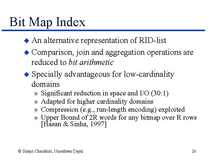
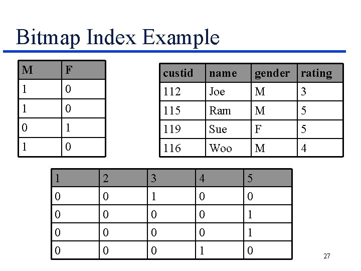
Bit Map Index u An alternative representation of RID-list u Comparison, join and aggregation operations are reduced to bit arithmetic u Specially advantageous for low-cardinality domains » » Significant reduction in space and I/O (30: 1) Adapted for higher cardinality domains Compression (e. g. , run-length encoding) exploited Upper Bound of 2 R words for any bitmap over R rows [Hasan & Sinha, 1997] © Surajit Chaudhuri, Umeshwar Dayal 26

Bitmap Index Example M F custid name gender rating 1 0 112 Joe M 3 1 0 115 Ram M 5 0 1 119 Sue F 5 1 0 116 Woo M 4 1 0 0 0 2 0 0 0 3 1 0 0 4 0 0 0 5 0 1 1 0 0 0 1 0 27

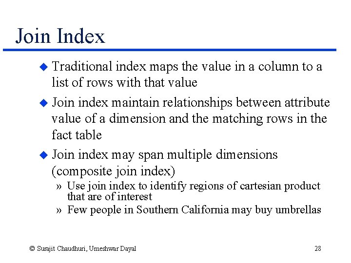
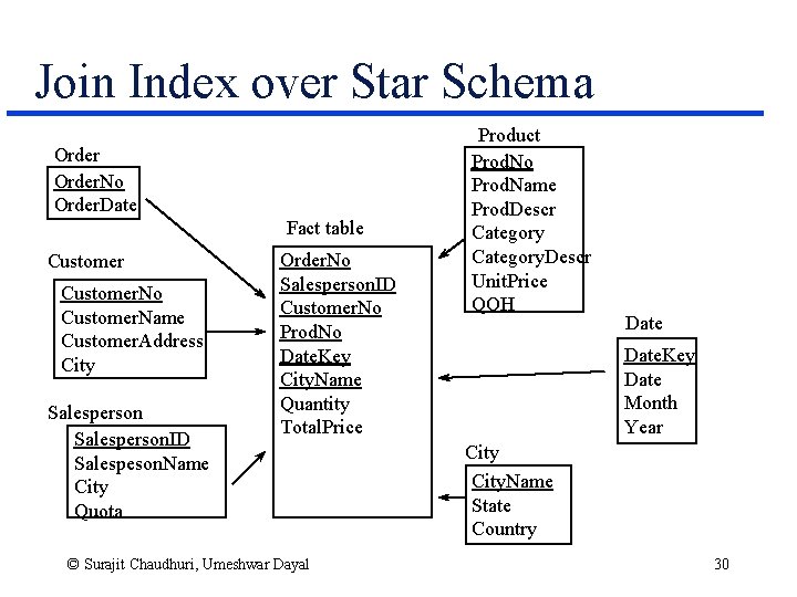
Join Index u Traditional index maps the value in a column to a list of rows with that value u Join index maintain relationships between attribute value of a dimension and the matching rows in the fact table u Join index may span multiple dimensions (composite join index) » Use join index to identify regions of cartesian product that are of interest » Few people in Southern California may buy umbrellas © Surajit Chaudhuri, Umeshwar Dayal 28

Algorithm Using Bitmapped Join Indexes u [O’Neil&Graefe 95] u Maintain bit mapped join indexes between each dimension table and the fact table u To answer a query over multiple dimensions » Take intersection of join indexes until the set of candidate fact tuples is small » Do foreign key joins with rest of the dimension tables » Look up the fact table © Surajit Chaudhuri, Umeshwar Dayal 29

Join Index over Star Schema Order. No Order. Date Fact table Customer. No Customer. Name Customer. Address City Salesperson. ID Salespeson. Name City Quota Order. No Salesperson. ID Customer. No Prod. No Date. Key City. Name Quantity Total. Price © Surajit Chaudhuri, Umeshwar Dayal Product Prod. No Prod. Name Prod. Descr Category. Descr Unit. Price QOH Date. Key Date Month Year City. Name State Country 30

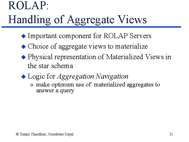
ROLAP: Handling of Aggregate Views u Important component for ROLAP Servers u Choice of aggregate views to materialize u Physical representation of Materialized Views in the star schema u Logic for Aggregation Navigation » make optimum use of materialized aggregates to answer a query © Surajit Chaudhuri, Umeshwar Dayal 31

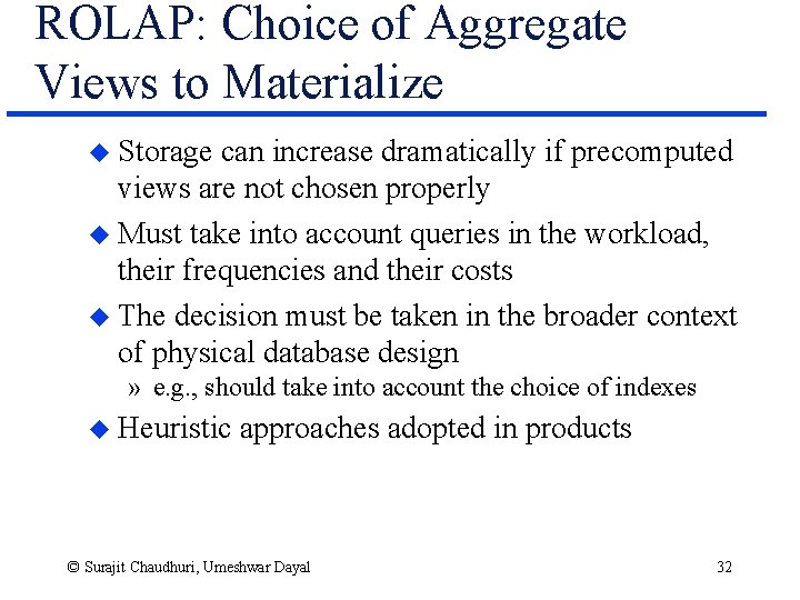
ROLAP: Choice of Aggregate Views to Materialize u Storage can increase dramatically if precomputed views are not chosen properly u Must take into account queries in the workload, their frequencies and their costs u The decision must be taken in the broader context of physical database design » e. g. , should take into account the choice of indexes u Heuristic approaches adopted in products © Surajit Chaudhuri, Umeshwar Dayal 32

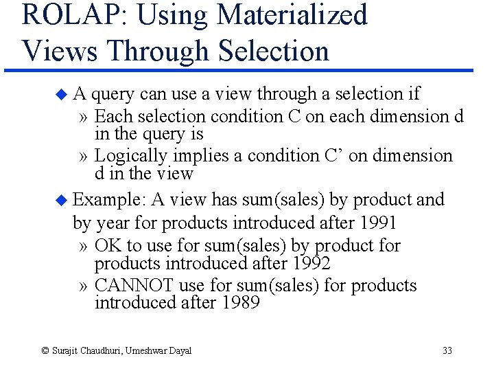
ROLAP: Using Materialized Views Through Selection u. A query can use a view through a selection if » Each selection condition C on each dimension d in the query is » Logically implies a condition C’ on dimension d in the view u Example: A view has sum(sales) by product and by year for products introduced after 1991 » OK to use for sum(sales) by product for products introduced after 1992 » CANNOT use for sum(sales) for products introduced after 1989 © Surajit Chaudhuri, Umeshwar Dayal 33

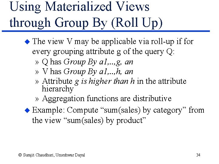
Using Materialized Views through Group By (Roll Up) u The view V may be applicable via roll-up if for every grouping attribute g of the query Q: » Q has Group By a 1, . . , g, an » V has Group By a 1, . . , h, an » Attribute g is higher than h in the attribute hierarchy » Aggregation functions are distributive u Example: Compute “sum(sales) by category” from the view “sum(sales) by product” © Surajit Chaudhuri, Umeshwar Dayal 34

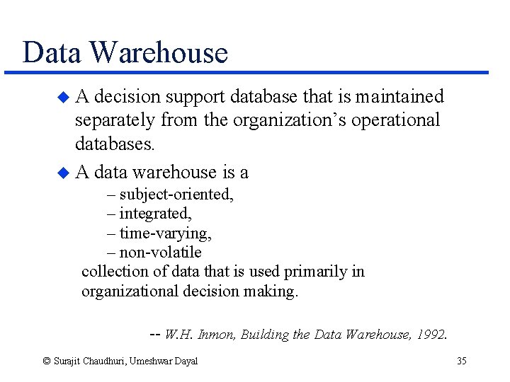
Data Warehouse u. A decision support database that is maintained separately from the organization’s operational databases. u A data warehouse is a – subject-oriented, – integrated, – time-varying, – non-volatile collection of data that is used primarily in organizational decision making. -- W. H. Inmon, Building the Data Warehouse, 1992. © Surajit Chaudhuri, Umeshwar Dayal 35

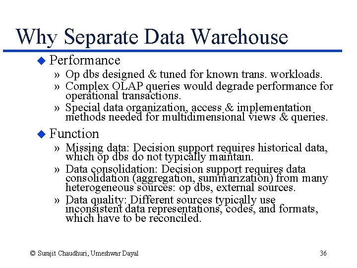
Why Separate Data Warehouse u Performance » Op dbs designed & tuned for known trans. workloads. » Complex OLAP queries would degrade performance for operational transactions. » Special data organization, access & implementation methods needed for multidimensional views & queries. u Function » Missing data: Decision support requires historical data, which op dbs do not typically maintain. » Data consolidation: Decision support requires data consolidation (aggregation, summarization) from many heterogeneous sources: op dbs, external sources. » Data quality: Different sources typically use inconsistent data representations, codes, and formats, which have to be reconciled. © Surajit Chaudhuri, Umeshwar Dayal 36

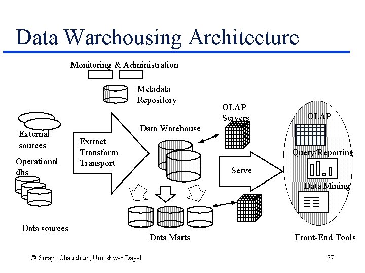
Data Warehousing Architecture Monitoring & Administration Metadata Repository External sources Operational dbs OLAP Servers OLAP Data Warehouse Extract Transform Transport Query/Reporting Serve Data Mining Data sources © Surajit Chaudhuri, Umeshwar Dayal Data Marts Front-End Tools 37

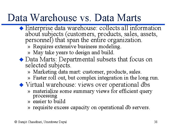
Data Warehouse vs. Data Marts u Enterprise data warehouse: collects all information about subjects (customers, products, sales, assets, personnel) that span the entire organization. » Requires extensive business modeling. » May take years to design and build. u Data Marts: Departmental subsets that focus on selected subjects. » Marketing data mart: customer, products, sales. » Faster roll out, but complex integration in the long run. u Virtual warehouse: views over operational dbs » materialize some summary views for efficient query processing » easier to build » requisite excess capacity on operational db servers. © Surajit Chaudhuri, Umeshwar Dayal 38

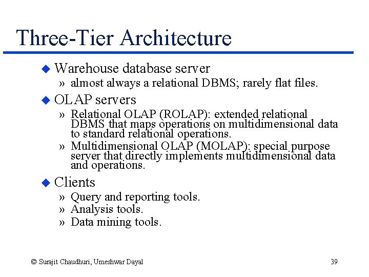
Three-Tier Architecture u Warehouse database server » almost always a relational DBMS; rarely flat files. u OLAP servers » Relational OLAP (ROLAP): extended relational DBMS that maps operations on multidimensional data to standard relational operations. » Multidimensional OLAP (MOLAP): special purpose server that directly implements multidimensional data and operations. u Clients » Query and reporting tools. » Analysis tools. » Data mining tools. © Surajit Chaudhuri, Umeshwar Dayal 39

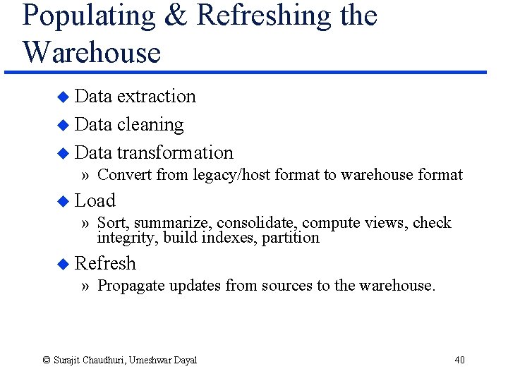
Populating & Refreshing the Warehouse u Data extraction u Data cleaning u Data transformation » Convert from legacy/host format to warehouse format u Load » Sort, summarize, consolidate, compute views, check integrity, build indexes, partition u Refresh » Propagate updates from sources to the warehouse. © Surajit Chaudhuri, Umeshwar Dayal 40

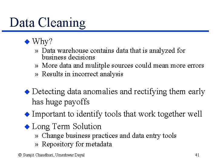
Data Cleaning u Why? » Data warehouse contains data that is analyzed for business decisions » More data and mulitple sources could mean more errors » Results in incorrect analysis u Detecting data anomalies and rectifying them early has huge payoffs u Important to identify tools that work together well u Long Term Solution » Change business practices and data entry tools » Repository for metadata © Surajit Chaudhuri, Umeshwar Dayal 41

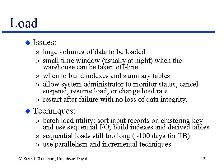
Load u Issues: » huge volumes of data to be loaded » small time window (usually at night) when the warehouse can be taken off-line » when to build indexes and summary tables » allow system administrator to monitor status, cancel suspend, resume load, or change load rate » restart after failure with no loss of data integrity. u Techniques: » batch load utility: sort input records on clustering key and use sequential I/O; build indexes and derived tables » sequential loads still too long (~100 days for TB) » use parallelism and incremental techniques. © Surajit Chaudhuri, Umeshwar Dayal 42

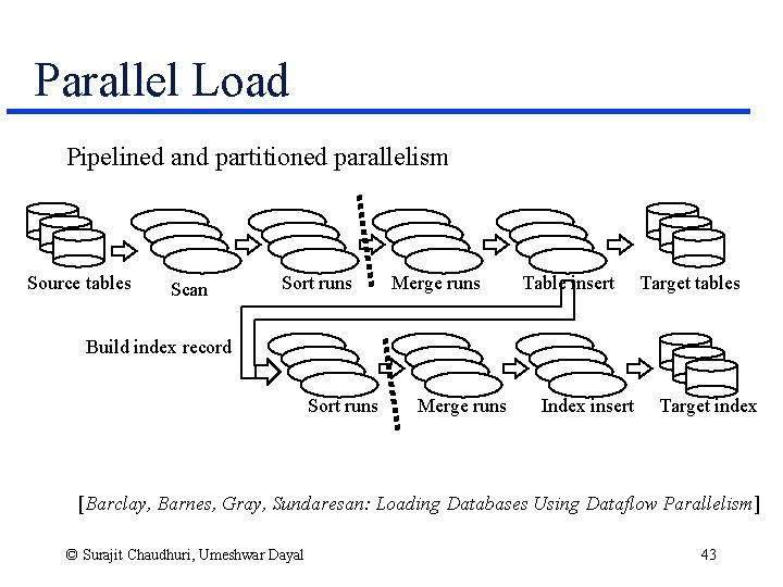
Parallel Load Pipelined and partitioned parallelism Source tables Scan Sort runs Merge runs Table insert Target tables Build index record Sort runs Merge runs Index insert Target index [Barclay, Barnes, Gray, Sundaresan: Loading Databases Using Dataflow Parallelism] © Surajit Chaudhuri, Umeshwar Dayal 43

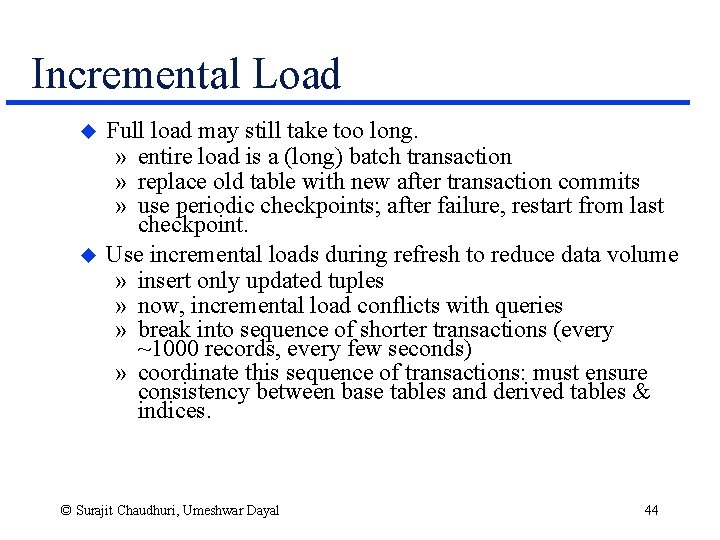
Incremental Load u u Full load may still take too long. » entire load is a (long) batch transaction » replace old table with new after transaction commits » use periodic checkpoints; after failure, restart from last checkpoint. Use incremental loads during refresh to reduce data volume » insert only updated tuples » now, incremental load conflicts with queries » break into sequence of shorter transactions (every ~1000 records, every few seconds) » coordinate this sequence of transactions: must ensure consistency between base tables and derived tables & indices. © Surajit Chaudhuri, Umeshwar Dayal 44

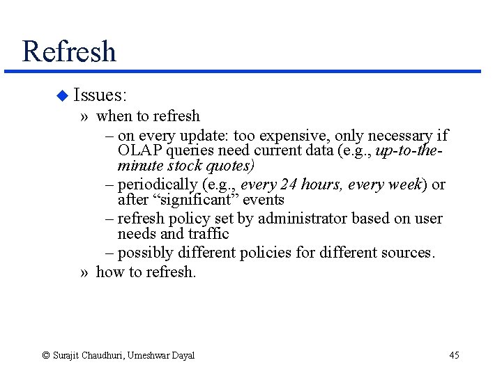
Refresh u Issues: » when to refresh – on every update: too expensive, only necessary if OLAP queries need current data (e. g. , up-to-theminute stock quotes) – periodically (e. g. , every 24 hours, every week) or after “significant” events – refresh policy set by administrator based on user needs and traffic – possibly different policies for different sources. » how to refresh. © Surajit Chaudhuri, Umeshwar Dayal 45

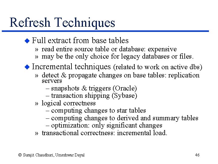
Refresh Techniques u Full extract from base tables » read entire source table or database: expensive » may be the only choice for legacy databases or files. u Incremental techniques (related to work on active dbs) » detect & propagate changes on base tables: replication servers – snapshots & triggers (Oracle) – transaction shipping (Sybase) » logical correctness – computing changes to star tables – computing changes to derived and summary tables – optimization: only significant changes » transactional correctness: incremental load. © Surajit Chaudhuri, Umeshwar Dayal 46