NTP Clock Discipline Principles David L Mills University

NTP Clock Discipline Principles David L. Mills University of Delaware http: //www. eecis. udel. edu/~mills mailto: mills@udel. edu Sir John Tenniel; Alice’s Adventures in Wonderland, Lewis Carroll 03 -Jun-21 1

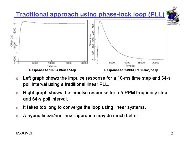
Traditional approach using phase-lock loop (PLL) Response to 10 -ms Phase Step Response to 2 -PPM Frequency Step o Left graph shows the impulse response for a 10 -ms time step and 64 -s poll interval using a traditional linear PLL. o Right graph shows the impulse response for a 5 -PPM frequency step and 64 -s poll interval. o It takes too long to converge the loop using linear systems. o A hybrid linear/nonlinear approach may do much better. 03 -Jun-21 2

Clock discipline design principles o The clock discipline algorithm functions as a nonlinear, hybrid phase/frequency-lock (NHPFL) feedback loop. o Detailed computer clock analysis yields the optimum averaging interval depending on prevailing network jitter and oscillator wander. o Optimum value is determined in real time by measuring the jitter and wander separately. o Clock state machine quickly converges time and frequency and suppresses transients resulting from leap events, etc. o Huff&puff algorithm corrects for large outlyers and asymmetric delays o Popcorn spike suppressor clips noise spikes. 03 -Jun-21 3

Clock discipline design approach o Phase noise due to network jitter prevails at the lower poll intervals, so a second-order phase-lock loop (PLL) is the best frequency predictor. o Frequency noise due to random-walk oscillator wander prevails at the higher poll intervals, so a first-order frequency-lock loop (FLL) is the best frequency predictor. o A crafted heuristic algorithm is necessary to combine both predictions. o The NHPFL algorithm combines the time and frequency predictions in a seamless way for poll intervals from 16 seconds to 36 hours. • The PLL frequency adjustment is computed as the integral of past frequency offsets. • The FLL frequency adjustment is computed as the exponential average of past frequency offsets. • An additional phase adjustment is necessary for loop stabiility. • The poll interval, which determines the loop time constant, is determined in response to measured jitter and wander. 6/3/2021 4

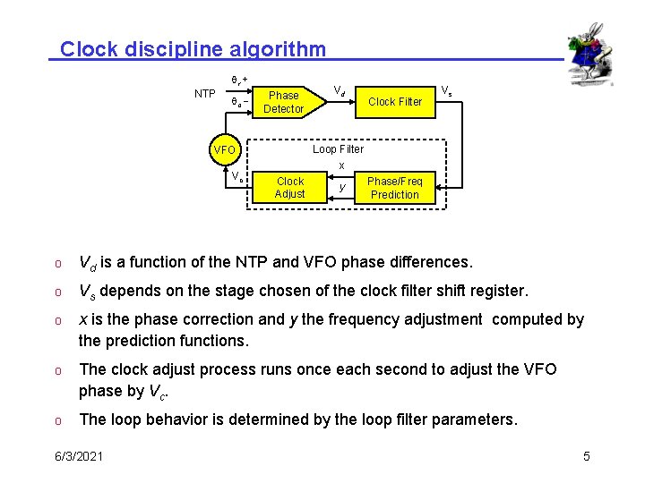
Clock discipline algorithm qr + NTP qc - Phase Detector Clock Filter Vs Loop Filter x VFO Vc Vd Clock Adjust y Phase/Freq Prediction o Vd is a function of the NTP and VFO phase differences. o Vs depends on the stage chosen of the clock filter shift register. o x is the phase correction and y the frequency adjustment computed by the prediction functions. o The clock adjust process runs once each second to adjust the VFO phase by Vc. o The loop behavior is determined by the loop filter parameters. 6/3/2021 5

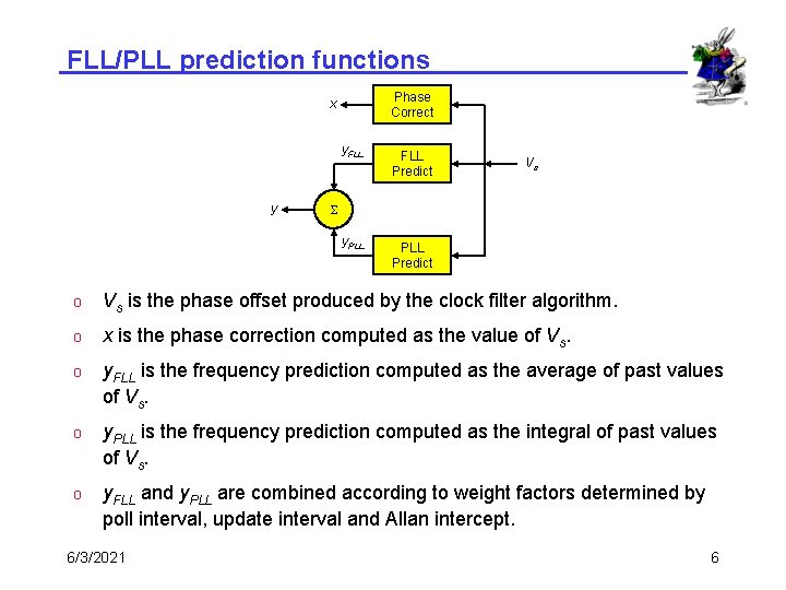
FLL/PLL prediction functions Phase Correct x y y. FLL Predict y. PLL Predict Vs S o Vs is the phase offset produced by the clock filter algorithm. o x is the phase correction computed as the value of Vs. o y. FLL is the frequency prediction computed as the average of past values of Vs. o y. PLL is the frequency prediction computed as the integral of past values of Vs. o y. FLL and y. PLL are combined according to weight factors determined by poll interval, update interval and Allan intercept. 6/3/2021 6

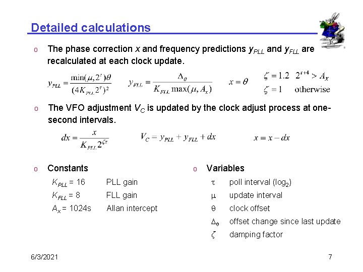
Detailed calculations o The phase correction x and frequency predictions y. PLL and y. FLL are recalculated at each clock update. o The VFO adjustment VC is updated by the clock adjust process at onesecond intervals. o Constants o Variables KPLL = 16 PLL gain t poll interval (log 2) KFLL = 8 FLL gain m update interval Ax = 1024 s Allan intercept q clock offset Dq offset change since last update ζ damping factor 6/3/2021 7

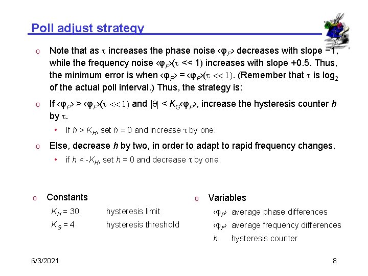
Poll adjust strategy o Note that as t increases the phase noise ‹φP› decreases with slope − 1, while the frequency noise ‹φF›(t << 1) increases with slope +0. 5. Thus, the minimum error is when ‹φP› = ‹φF›(t << 1). (Remember that t is log 2 of the actual poll interval. ) Thus, the strategy is: o If ‹φP› > ‹φF›(t << 1) and |q| < KG‹φP›, increase the hysteresis counter h by t. • o Else, decrease h by two, in order to adapt to rapid frequency changes. • o If h > KH, set h = 0 and increase t by one. if h < -KH, set h = 0 and decrease t by one. Constants o Variables KH = 30 hysteresis limit ‹φP› average phase differences KG = 4 hysteresis threshold ‹φF› average frequency differences h 6/3/2021 hysteresis counter 8

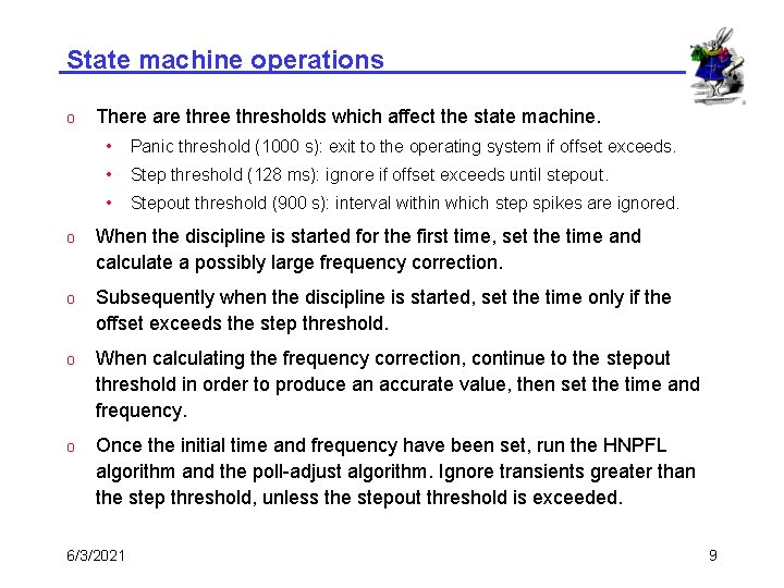
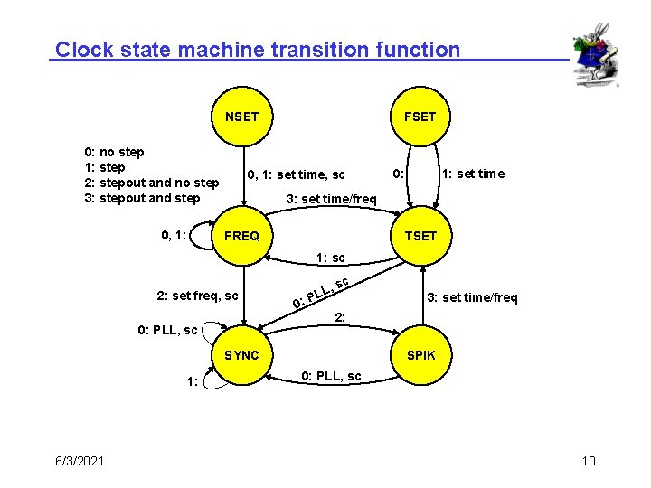
State machine operations o There are thresholds which affect the state machine. • Panic threshold (1000 s): exit to the operating system if offset exceeds. • Step threshold (128 ms): ignore if offset exceeds until stepout. • Stepout threshold (900 s): interval within which step spikes are ignored. o When the discipline is started for the first time, set the time and calculate a possibly large frequency correction. o Subsequently when the discipline is started, set the time only if the offset exceeds the step threshold. o When calculating the frequency correction, continue to the stepout threshold in order to produce an accurate value, then set the time and frequency. o Once the initial time and frequency have been set, run the HNPFL algorithm and the poll-adjust algorithm. Ignore transients greater than the step threshold, unless the stepout threshold is exceeded. 6/3/2021 9

Clock state machine transition function NSET 0: no step 1: step 2: stepout and no step 3: stepout and step 0, 1: FSET 0, 1: set time, sc 0: 1: set time 3: set time/freq FREQ TSET 1: sc 2: set freq, sc 0: PLL, sc 0: , sc L PL 2: SYNC 1: 6/3/2021 3: set time/freq SPIK 0: PLL, sc 10

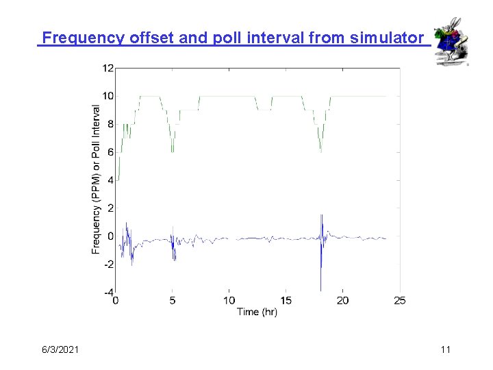
Frequency offset and poll interval from simulator 6/3/2021 11

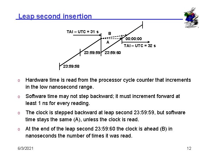
Leap second insertion TAI – UTC = 31 s B A 23: 59 00: 00 TAI – UTC = 32 s 23: 59: 60 23: 59: 58 o Hardware time is read from the processor cycle counter that increments in the low nanosecond range. o Software time may not step backward; it must increment forward at least 1 ns for every reading. o The clock is stepped backward at leap second 23: 59, but software time stays the same (A), unless the clock is read. o At the end of the leap second 23: 59: 60 the clock is ahead (B) in nanoseconds the number of times it was read. 6/3/2021 12

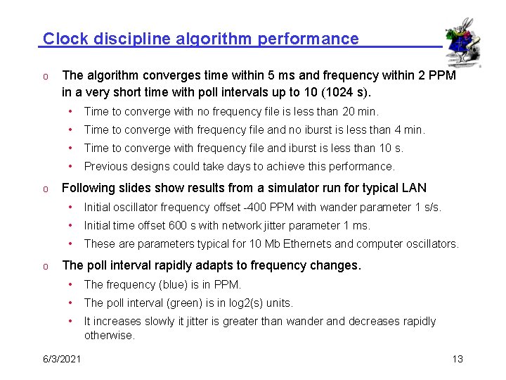
Clock discipline algorithm performance o o o The algorithm converges time within 5 ms and frequency within 2 PPM in a very short time with poll intervals up to 10 (1024 s). • Time to converge with no frequency file is less than 20 min. • Time to converge with frequency file and no iburst is less than 4 min. • Time to converge with frequency file and iburst is less than 10 s. • Previous designs could take days to achieve this performance. Following slides show results from a simulator run for typical LAN • Initial oscillator frequency offset -400 PPM with wander parameter 1 s/s. • Initial time offset 600 s with network jitter parameter 1 ms. • These are parameters typical for 10 Mb Ethernets and computer oscillators. The poll interval rapidly adapts to frequency changes. • The frequency (blue) is in PPM. • The poll interval (green) is in log 2(s) units. • It increases slowly it jitter is greater than wander and decreases rapidly otherwise. 6/3/2021 13

Further information o o NTP home page http: //www. ntp. org • Current NTP Version 3 and 4 software and documentation • FAQ and links to other sources and interesting places David L. Mills home page http: //www. eecis. udel. edu/~mills • Papers, reports and memoranda in Post. Script and PDF formats • Briefings in HTML, Post. Script, Power. Point and PDF formats • Collaboration resources hardware, software and documentation • Songs, photo galleries and after-dinner speech scripts Udel FTP server: ftp: //ftp. udel. edu/pub/ntp • Current NTP Version software, documentation and support • Collaboration resources and junkbox Related projects http: //www. eecis. udel. edu/~mills/status. htm • Current research project descriptions and briefings 03 -Jun-21 14