Multidisciplinary Optimization of Composite Laminates with Resin Transfer

Multidisciplinary Optimization of Composite Laminates with Resin Transfer Molding Chung-Hae PARK

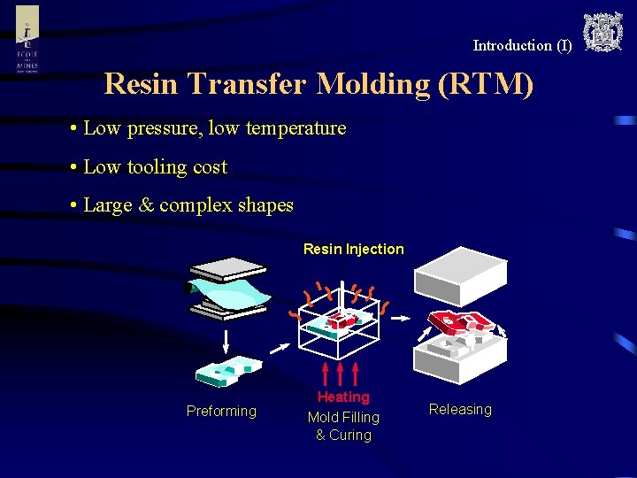
Introduction (I) Resin Transfer Molding (RTM) • Low pressure, low temperature • Low tooling cost • Large & complex shapes Resin Injection Preforming Heating Mold Filling & Curing Releasing

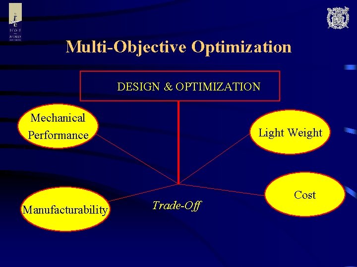
Multi-Objective Optimization DESIGN & OPTIMIZATION Mechanical Performance Manufacturability Light Weight Trade-Off Cost

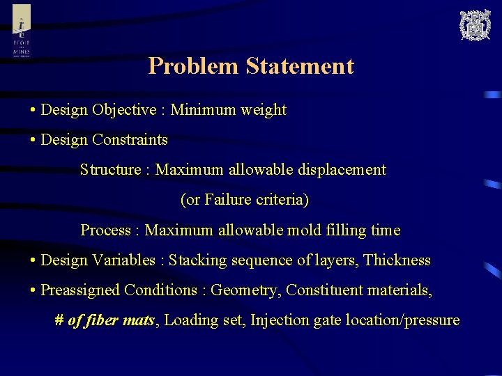
Problem Statement • Design Objective : Minimum weight • Design Constraints Structure : Maximum allowable displacement (or Failure criteria) Process : Maximum allowable mold filling time • Design Variables : Stacking sequence of layers, Thickness • Preassigned Conditions : Geometry, Constituent materials, # of fiber mats, Loading set, Injection gate location/pressure

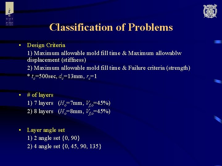
Classification of Problems • Design Criteria 1) Maximum allowable mold fill time & Maximum allowablw displacement (stiffness) 2) Maximum allowable mold fill time & Failure criteria (strength) * tc=500 sec, dc=13 mm, rc=1 • # of layers 1) 7 layers (Ho=7 mm, Vf, o=45%) 2) 8 layers (Ho=8 mm, Vf, o=45%) • Layer angle set 1) 2 angle set {0, 90} 2) 4 angle set {0, 45, 90, 135}

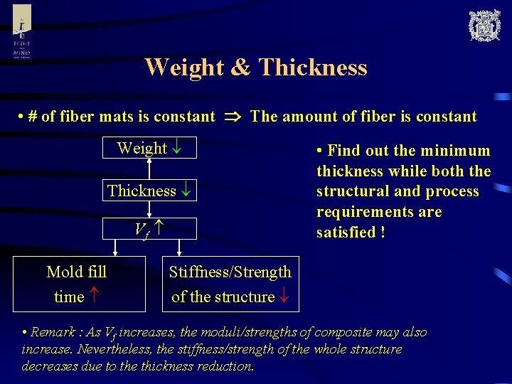
Weight & Thickness • # of fiber mats is constant The amount of fiber is constant Weight Thickness Vf Mold fill time • Find out the minimum thickness while both the structural and process requirements are satisfied ! Stiffness/Strength of the structure • Remark : As Vf increases, the moduli/strengths of composite may also increase. Nevertheless, the stiffness/strength of the whole structure decreases due to the thickness reduction.

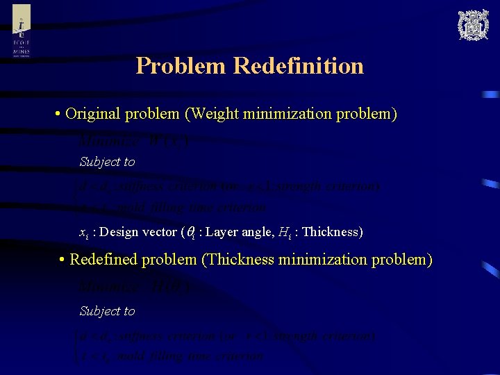
Problem Redefinition • Original problem (Weight minimization problem) Subject to xi : Design vector ( i : Layer angle, Hi : Thickness) • Redefined problem (Thickness minimization problem) Subject to

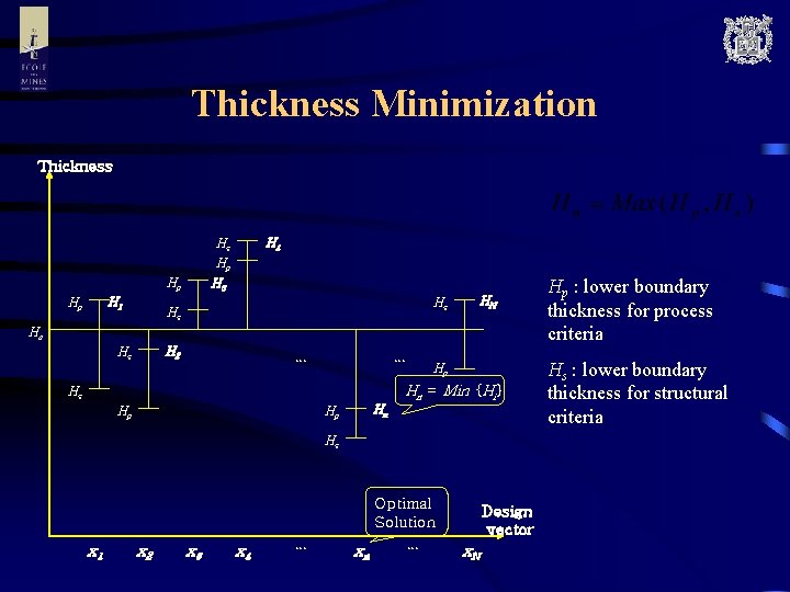
Thickness Minimization Thickness Hs Hp H 3 Hp Hp H 1 H 4 Hs Hs HN Ho H 2 Hs … … Hp Hn = Min {Hi} Hs Hp Hn Hp Hs Optimal Solution x 1 x 2 x 3 x 4 … xn … Design vector x. N Hp : lower boundary thickness for process criteria Hs : lower boundary thickness for structural criteria

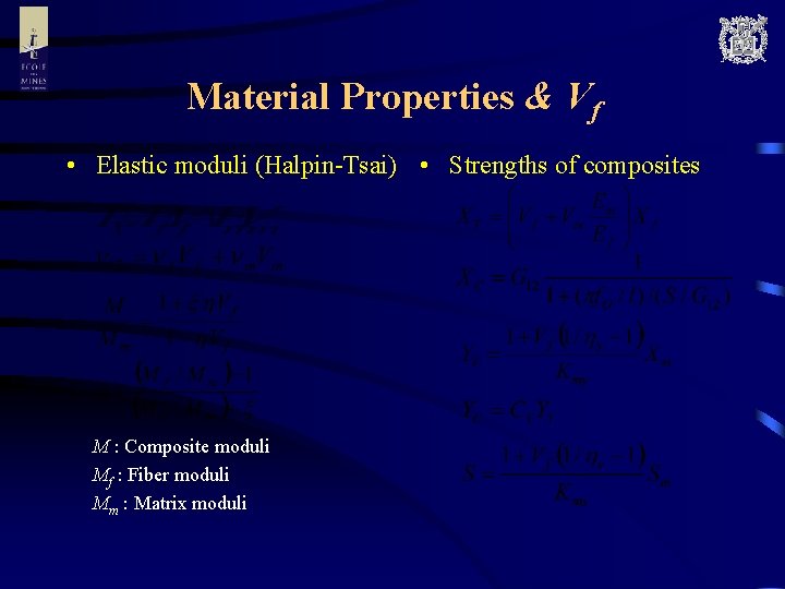
Material Properties & Vf • Elastic moduli (Halpin-Tsai) • Strengths of composites M : Composite moduli Mf : Fiber moduli Mm : Matrix moduli

Mathematical Models (I) Structural Analysis • Classical Lamination Theory • Finite Element Calculation FEAD-LASP with 16 serendip elements • Tsai-Wu Failure Criteria If r >1 : Failure

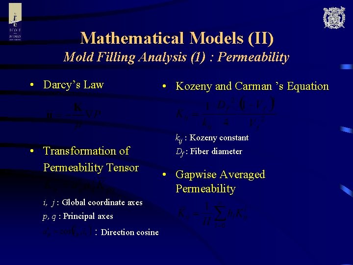
Mathematical Models (II) Mold Filling Analysis (1) : Permeability • Darcy’s Law • Transformation of Permeability Tensor i, j : Global coordinate axes p, q : Principal axes : Direction cosine • Kozeny and Carman ’s Equation kij : Kozeny constant Df : Fiber diameter • Gapwise Averaged Permeability

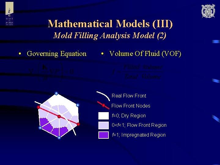
Mathematical Models (III) Mold Filling Analysis Model (2) • Governing Equation • Volume Of Fluid (VOF) Real Flow Front Nodes f=0; Dry Region 0<f<1; Flow Front Region f=1; Impregnated Region

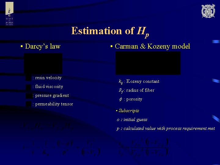
Estimation of Hp • Darcy’s law : resin velocity : fluid viscosity : pressure gradient : permeability tensor • Carman & Kozeny model kij : Kozeny constant Rf : radius of fiber : porosity • Subscripts o : initial guess p : calculated value with process requirement met

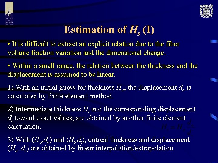
Estimation of Hs (I) • It is difficult to extract an explicit relation due to the fiber volume fraction variation and the dimensional change. • Within a small range, the relation between the thickness and the displacement is assumed to be linear. 1) With an initial guess for thickness Ho, the displacement do is calculated by finite element method. 2) Intermediate thickness Ht and the corresponding displacement dt toward exact values, are obtained by another finite element calculation. 3) With (Ho, do) and (Ht, dt), critical thickness and displacement (Hs, dc) are obtained by linear interpolation/extrapolation.

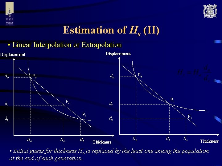
Estimation of Hs (II) • Linear Interpolation or Extrapolation Displacement do Po Ps dc Hs Pt dt Ho Po do Ht Ps dc Thickness Ho Ht Hs Thickness • Initial guess for thickness Ho is replaced by the least one among the population at the end of each generation.

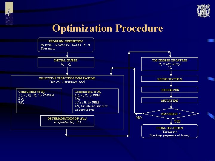
Optimization Procedure PROBLEM DEFINITION Material, Geometry, Loads, # of fiber mats INITIAL GUESS THICKNESS UPDATING Ho , Vfo Ho = Min (H(xi)) Vfo OBJECTIVE FUNCTION EVALUATION (for i=1, Population size) Computation of Hp 1 to at Vfo, Ho by CVFEM 2 Vfp 3 Hp REPRODUCTION CROSSOVER Computation of Hs 1 do at Ho by FEM 2 Ht 3 dt at Ht by FEM 4 Hs by interpolation(or extrapolation) MUTATION CONVERGE ? DETERMINATION OF H(xi)=Max (Hp, Hs) NO YES FINAL SOLUTION Thickness Stacking sequence of layers

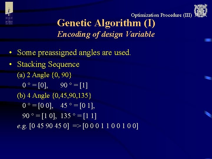
Optimization Procedure (III) Genetic Algorithm (I) Encoding of design Variable • Some preassigned angles are used. • Stacking Sequence (a) 2 Angle {0, 90} 0 ° = [0], 90 ° = [1] (b) 4 Angle {0, 45, 90, 135} 0 ° = [0 0], 45 ° = [0 1], 90 ° = [1 0], 135 ° = [1 1] e. g. [0 45 90 45 0] => [0 0 0 1 1 0 0]

Optimization Procedure (IV) Genetic Algorithm (II) Genetic Operators • Reproduction Selection of the fitter members into a mating pool Probability of selection • Crossover Parent 1 = 1101100 | 010 Parent 2 = 0111011 | 110 Child 1 = 110110 Child 2 = 0111011010 • Mutation Switch from 0 to 1 or vice versa at a randomly chosen location on a binary string Elitism : The best individual of the population is preserved without crossover nor mutation, in order to prevent from losing the best individual of the population and to improve the efficiency of the genetic search

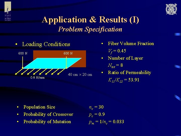
Application & Results (I) Problem Specification • Loading Conditions 500 N 0. 8 N/mm 40 cm 20 cm • Population Size • Probability of Crossover • Probability of Mutation • Fiber Volume Fraction Vf = 0. 45 • Number of Layer Ntot = 8 • Ratio of Permeability K 11/K 22 = 53. 91 nc = 30 pc = 0. 9 pm = 1/nc = 0. 033

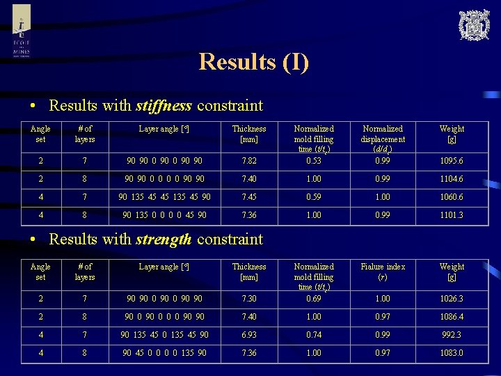
Results (I) • Results with stiffness constraint Angle set # of layers Layer angle [ ] Thickness [mm] Normalized displacement (d/dc) 0. 99 Weight [g] 7. 82 Normalized mold filling time (t/tc) 0. 53 2 7 90 90 90 2 8 90 90 0 0 90 90 7. 40 1. 00 0. 99 1104. 6 4 7 90 135 45 45 135 45 90 7. 45 0. 59 1. 00 1060. 6 4 8 90 135 0 0 45 90 7. 36 1. 00 0. 99 1101. 3 Fialure index (r) Weight [g] 1. 00 1026. 3 1095. 6 • Results with strength constraint Angle set # of layers Layer angle [ ] Thickness [mm] 2 7 90 90 90 7. 30 Normalized mold filling time (t/tc) 0. 69 2 8 90 0 0 0 90 90 7. 40 1. 00 0. 97 1086. 4 4 7 90 135 45 90 6. 93 0. 74 0. 99 992. 3 4 8 90 45 0 0 135 90 7. 36 1. 00 0. 97 1083. 0

Results (II) • Results with stiffness constraint & 2 angle set Thickness [mm] Design Criteria Results of 2 Angle Set and 7 Layers Thickness [mm] Design Criteria Results of 2 Angle Set and 8 Layers

Results (III) • Results with stiffness constraint & 4 angle set Thickness [mm] Design Criteria Results of 4 Angle Set and 7 Layers Thickness [mm] Design Criteria Results of 4 Angle Set and 8 Layers

Results (IV) • Results with strength constraint & 2 angle set Thickness [mm] Design Criteria Results of 2 Angle Set and 7 Layers Thickness [mm] Design Criteria Results of 2 Angle Set and 8 Layers

Results (V) • Results with strength constraint & 4 angle set Thickness [mm] Design Criteria Results of 4 Angle Set and 7 Layers Thickness [mm] Design Criteria Results of 4 Angle Set and 8 Layers

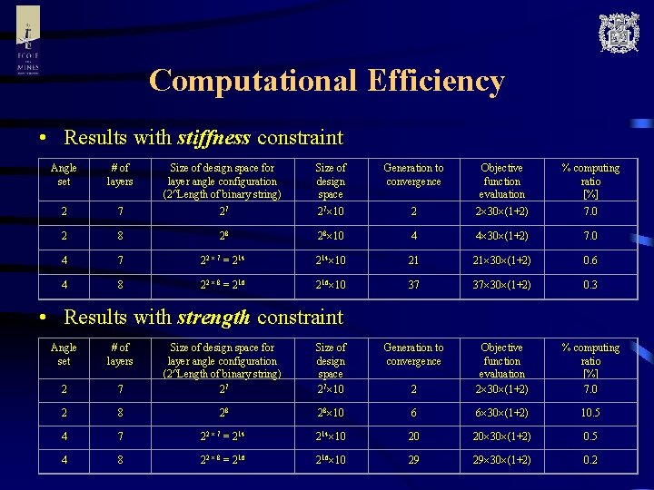
Computational Efficiency • Results with stiffness constraint Angle set # of layers Size of design space for layer angle configuration (2^Length of binary string) Size of design space Generation to convergence Objective function evaluation % computing ratio [%] 2 7 27 27 10 2 2 30 (1+2) 7. 0 2 8 28 28 10 4 4 30 (1+2) 7. 0 4 7 22 7 = 214 10 21 21 30 (1+2) 0. 6 4 8 22 8 = 216 10 37 37 30 (1+2) 0. 3 % computing ratio [%] 7. 0 • Results with strength constraint Angle set # of layers Size of design space 27 10 Generation to convergence 7 Size of design space for layer angle configuration (2^Length of binary string) 27 2 Objective function evaluation 2 30 (1+2) 2 2 8 28 28 10 6 6 30 (1+2) 10. 5 4 7 22 7 = 214 10 20 20 30 (1+2) 0. 5 4 8 22 8 = 216 10 29 29 30 (1+2) 0. 2

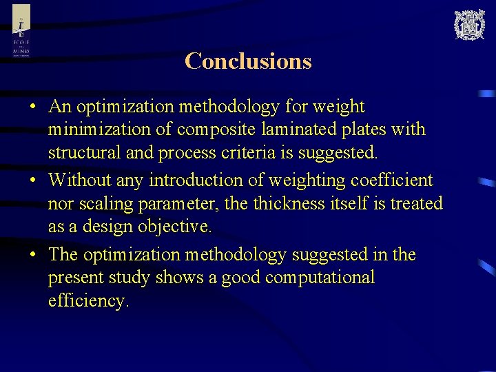
Conclusions • An optimization methodology for weight minimization of composite laminated plates with structural and process criteria is suggested. • Without any introduction of weighting coefficient nor scaling parameter, the thickness itself is treated as a design objective. • The optimization methodology suggested in the present study shows a good computational efficiency.