More on Recursion 2006 Pearson AddisonWesley All rights

More on Recursion © 2006 Pearson Addison-Wesley. All rights reserved 1

Backtracking • Backtracking – A strategy for guessing at a solution and backing up when an impasse is reached • Recursion and backtracking can be combined to solve problems © 2006 Pearson Addison-Wesley. All rights reserved 2

The Eight Queens Problem • Problem – Place eight queens on the chessboard so that no queen can attack any other queen • Strategy: guess at a solution – There are 4, 426, 165, 368 ways to arrange 8 queens on a chessboard of 64 squares © 2006 Pearson Addison-Wesley. All rights reserved 3

The Eight Queens Problem • An observation that eliminates many arrangements from consideration – No queen can reside in a row or a column that contains another queen • Now: only 40, 320 arrangements of queens to be checked for attacks along diagonals © 2006 Pearson Addison-Wesley. All rights reserved 4

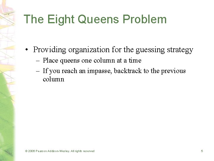
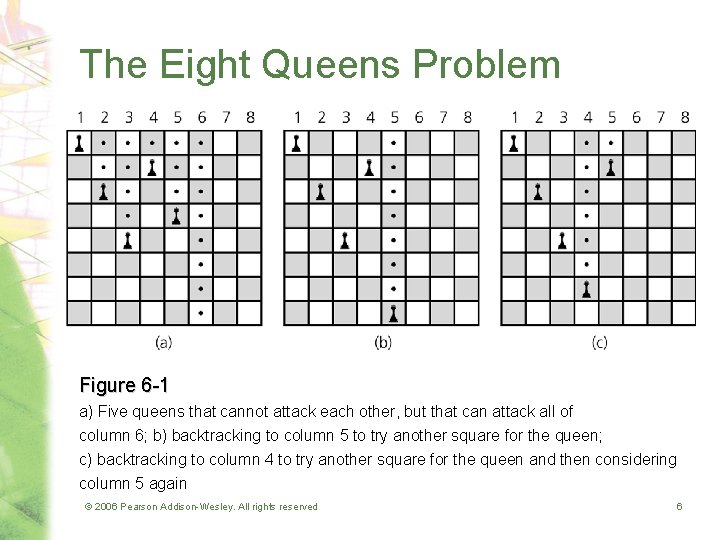
The Eight Queens Problem • Providing organization for the guessing strategy – Place queens one column at a time – If you reach an impasse, backtrack to the previous column © 2006 Pearson Addison-Wesley. All rights reserved 5

The Eight Queens Problem Figure 6 -1 a) Five queens that cannot attack each other, but that can attack all of column 6; b) backtracking to column 5 to try another square for the queen; c) backtracking to column 4 to try another square for the queen and then considering column 5 again © 2006 Pearson Addison-Wesley. All rights reserved 6

The Eight Queens Problem • A recursive algorithm that places a queen in a column – Base case • If there are no more columns to consider – You are finished – Recursive step • If you successfully place a queen in the current column – Consider the next column • If you cannot place a queen in the current column – You need to backtrack © 2006 Pearson Addison-Wesley. All rights reserved 7

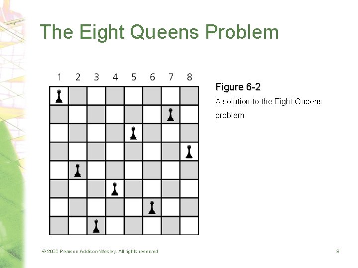
The Eight Queens Problem Figure 6 -2 A solution to the Eight Queens problem © 2006 Pearson Addison-Wesley. All rights reserved 8

The Relationship Between Recursion and Mathematical Induction • A strong relationship exists between recursion and mathematical induction • Induction can be used to – Prove properties about recursive algorithms – Prove that a recursive algorithm performs a certain amount of work © 2006 Pearson Addison-Wesley. All rights reserved 9

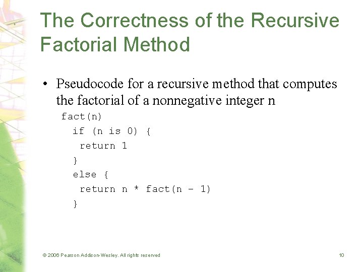
The Correctness of the Recursive Factorial Method • Pseudocode for a recursive method that computes the factorial of a nonnegative integer n fact(n) if (n is 0) { return 1 } else { return n * fact(n – 1) } © 2006 Pearson Addison-Wesley. All rights reserved 10

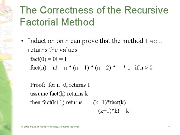
The Correctness of the Recursive Factorial Method • Induction on n can prove that the method fact returns the values fact(0) = 0! = 1 fact(n) = n! = n * (n – 1) * (n – 2) * …* 1 if n > 0 Proof: for n=0, returns 1 assume fact(k) returns k! then fact(k+1) returns (k+1)*fact(k) = (k+1)*k! = k! © 2006 Pearson Addison-Wesley. All rights reserved 11

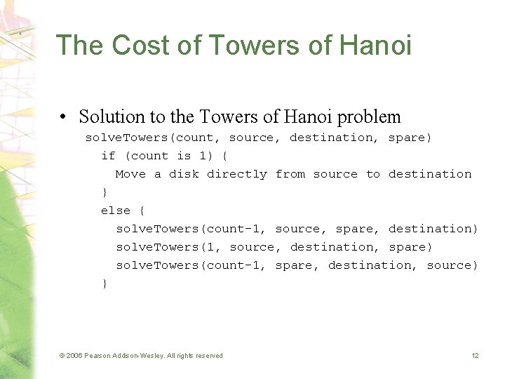
The Cost of Towers of Hanoi • Solution to the Towers of Hanoi problem solve. Towers(count, source, destination, spare) if (count is 1) { Move a disk directly from source to destination } else { solve. Towers(count-1, source, spare, destination) solve. Towers(1, source, destination, spare) solve. Towers(count-1, spare, destination, source) } © 2006 Pearson Addison-Wesley. All rights reserved 12

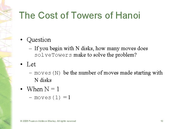
The Cost of Towers of Hanoi • Question – If you begin with N disks, how many moves does solve. Towers make to solve the problem? • Let – moves(N) be the number of moves made starting with N disks • When N = 1 – moves(1) = 1 © 2006 Pearson Addison-Wesley. All rights reserved 13

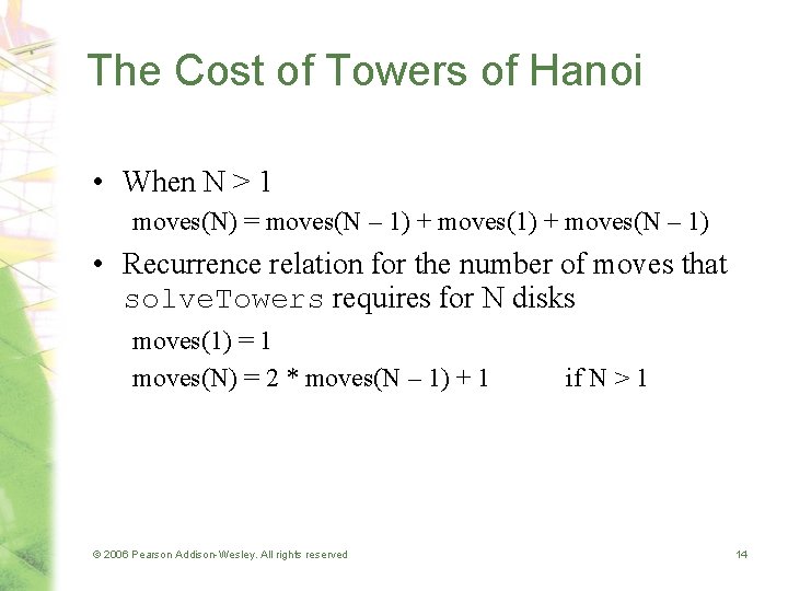
The Cost of Towers of Hanoi • When N > 1 moves(N) = moves(N – 1) + moves(N – 1) • Recurrence relation for the number of moves that solve. Towers requires for N disks moves(1) = 1 moves(N) = 2 * moves(N – 1) + 1 © 2006 Pearson Addison-Wesley. All rights reserved if N > 1 14

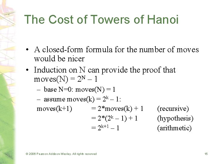
The Cost of Towers of Hanoi • A closed-formula for the number of moves would be nicer • Induction on N can provide the proof that moves(N) = 2 N – 1 – base N=0: moves(N) = 1 – assume moves(k) = 2 k – 1: moves(k+1) = 2*moves(k) + 1 = 2*(2 k – 1) + 1 = 2 k+1 – 1 © 2006 Pearson Addison-Wesley. All rights reserved (recursive) (hypothesis) (arithmetic) 15

Algorithm Efficiency © 2006 Pearson Addison-Wesley. All rights reserved 16

Measuring the Efficiency of Algorithms • Analysis of algorithms – Provides tools for contrasting the efficiency of different methods of solution • A comparison of algorithms – Should focus of significant differences in efficiency – Should not consider reductions in computing costs due to clever coding tricks © 2006 Pearson Addison-Wesley. All rights reserved 17

Measuring the Efficiency of Algorithms • Three difficulties with comparing programs instead of algorithms – How are the algorithms coded? – What computer should you use? – What data should the programs use? • Algorithm analysis should be independent of – Specific implementations – Computers – Data © 2006 Pearson Addison-Wesley. All rights reserved 18

The Execution Time of Algorithms • Counting an algorithm's operations is a way to access its efficiency – An algorithm’s execution time is related to the number of operations it requires – Examples • The Towers of Hanoi • Nested Loops © 2006 Pearson Addison-Wesley. All rights reserved 19

Actual Running Time • Consider the following pseudocode algorithm: Given input n int[] n_by_n = new int[n][n]; for i<n, j<n set n_by_n[i][j] = random(); print “The random array is created”; © 2006 Pearson Addison-Wesley. All rights reserved 20

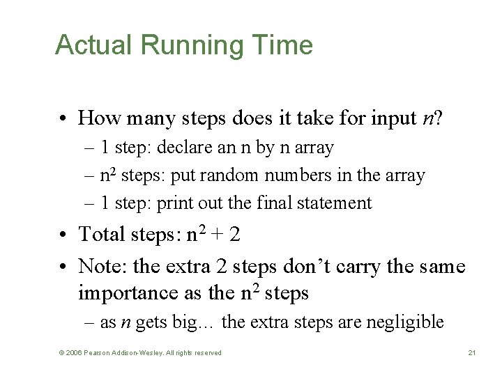
Actual Running Time • How many steps does it take for input n? – 1 step: declare an n by n array – n 2 steps: put random numbers in the array – 1 step: print out the final statement • Total steps: n 2 + 2 • Note: the extra 2 steps don’t carry the same importance as the n 2 steps – as n gets big… the extra steps are negligible © 2006 Pearson Addison-Wesley. All rights reserved 21

Actual Running Time • We also think of constants as negligible – we want to say n 2 and c*n 2 have “essentially” the same running time as n increases – more accurately: the same asymptotic running time • Commercial programmers would argue here… constants can matter in practice © 2006 Pearson Addison-Wesley. All rights reserved 22

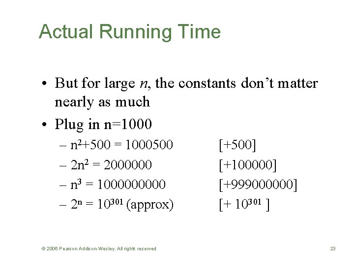
Actual Running Time • But for large n, the constants don’t matter nearly as much • Plug in n=1000 – n 2+500 = 1000500 – 2 n 2 = 2000000 – n 3 = 100000 – 2 n = 10301 (approx) © 2006 Pearson Addison-Wesley. All rights reserved [+500] [+100000] [+999000000] [+ 10301 ] 23

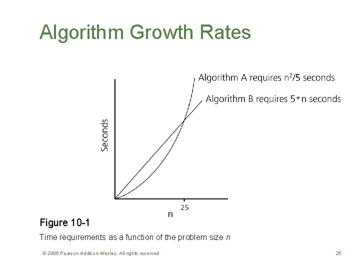
Algorithm Growth Rates • An algorithm’s time requirements can be measured as a function of the problem size • An algorithm’s growth rate – Enables the comparison of one algorithm with another – Examples Algorithm A requires time proportional to n 2 Algorithm B requires time proportional to n • Algorithm efficiency is typically a concern for large problems only © 2006 Pearson Addison-Wesley. All rights reserved 24

Algorithm Growth Rates Figure 10 -1 Time requirements as a function of the problem size n © 2006 Pearson Addison-Wesley. All rights reserved 25

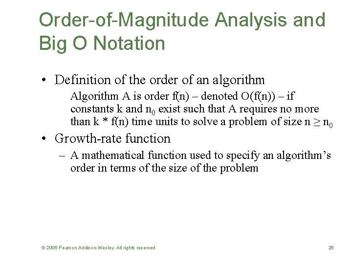
Order-of-Magnitude Analysis and Big O Notation • Definition of the order of an algorithm A is order f(n) – denoted O(f(n)) – if constants k and n 0 exist such that A requires no more than k * f(n) time units to solve a problem of size n ≥ n 0 • Growth-rate function – A mathematical function used to specify an algorithm’s order in terms of the size of the problem © 2006 Pearson Addison-Wesley. All rights reserved 26

Big O Notation • Running time will be measured with Big-O notation • Big-O is a way to indicate how fast a function grows © 2006 Pearson Addison-Wesley. All rights reserved 27

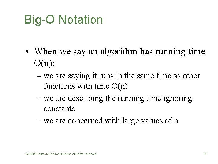
Big-O Notation • When we say an algorithm has running time O(n): – we are saying it runs in the same time as other functions with time O(n) – we are describing the running time ignoring constants – we are concerned with large values of n © 2006 Pearson Addison-Wesley. All rights reserved 28

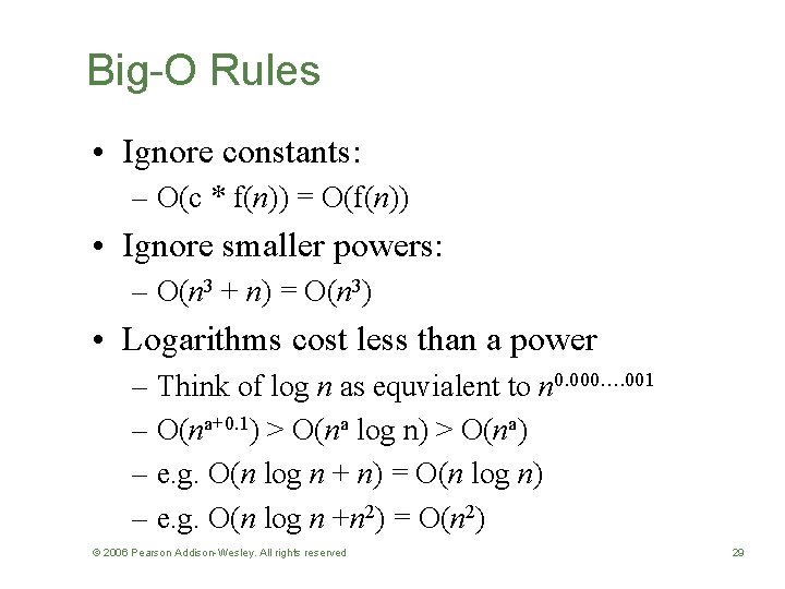
Big-O Rules • Ignore constants: – O(c * f(n)) = O(f(n)) • Ignore smaller powers: – O(n 3 + n) = O(n 3) • Logarithms cost less than a power – Think of log n as equvialent to n 0. 000…. 001 – O(na+0. 1) > O(na log n) > O(na) – e. g. O(n log n + n) = O(n log n) – e. g. O(n log n +n 2) = O(n 2) © 2006 Pearson Addison-Wesley. All rights reserved 29

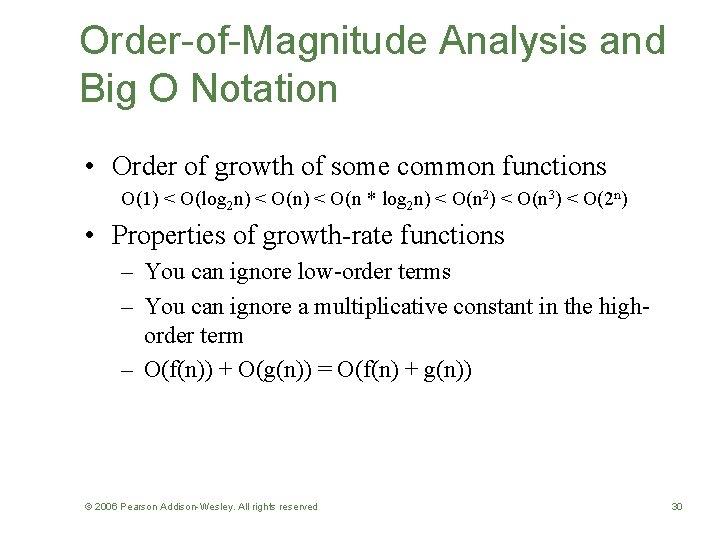
Order-of-Magnitude Analysis and Big O Notation • Order of growth of some common functions O(1) < O(log 2 n) < O(n * log 2 n) < O(n 2) < O(n 3) < O(2 n) • Properties of growth-rate functions – You can ignore low-order terms – You can ignore a multiplicative constant in the highorder term – O(f(n)) + O(g(n)) = O(f(n) + g(n)) © 2006 Pearson Addison-Wesley. All rights reserved 30

Why Big-O? • Look at what happens for large inputs – small problems are easy to do quickly – big problems are more interesting – larger function makes a huge difference for big n • Ignores irrelevant details – Constants and lower order terms depend on implementation… Big-O focuses on the algorithm © 2006 Pearson Addison-Wesley. All rights reserved 31

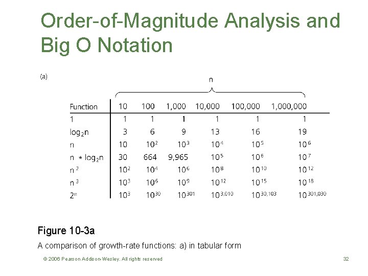
Order-of-Magnitude Analysis and Big O Notation Figure 10 -3 a A comparison of growth-rate functions: a) in tabular form © 2006 Pearson Addison-Wesley. All rights reserved 32

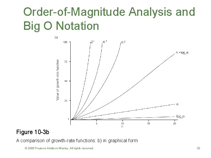
Order-of-Magnitude Analysis and Big O Notation Figure 10 -3 b A comparison of growth-rate functions: b) in graphical form © 2006 Pearson Addison-Wesley. All rights reserved 33

Determining Running Time • Need to count the number of “steps” to complete – need to consider the worst case – for input of size n – a “step” must take constant (O(1)) time • Often: – iterations of the inner loop * work per loop – recursive calls * work per call © 2006 Pearson Addison-Wesley. All rights reserved 34

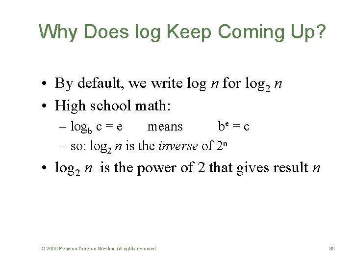
Why Does log Keep Coming Up? • By default, we write log n for log 2 n • High school math: – logb c = e means be = c – so: log 2 n is the inverse of 2 n • log 2 n is the power of 2 that gives result n © 2006 Pearson Addison-Wesley. All rights reserved 35

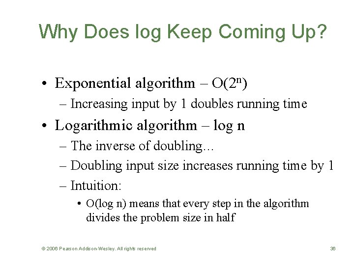
Why Does log Keep Coming Up? • Exponential algorithm – O(2 n) – Increasing input by 1 doubles running time • Logarithmic algorithm – log n – The inverse of doubling… – Doubling input size increases running time by 1 – Intuition: • O(log n) means that every step in the algorithm divides the problem size in half © 2006 Pearson Addison-Wesley. All rights reserved 36

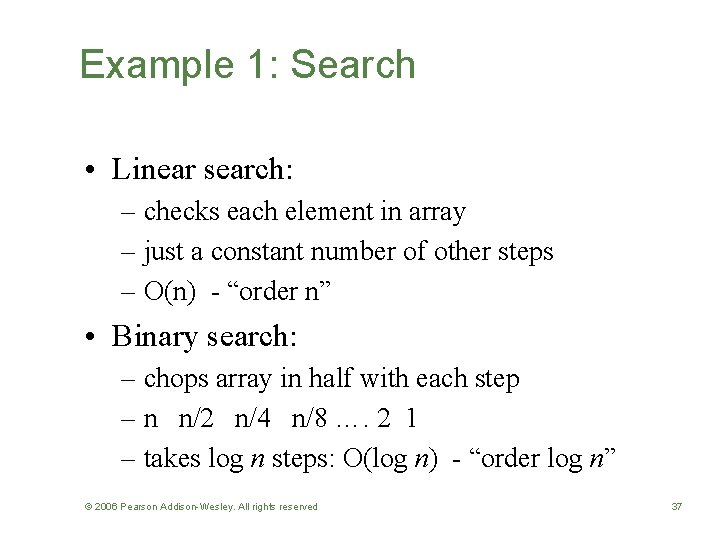
Example 1: Search • Linear search: – checks each element in array – just a constant number of other steps – O(n) - “order n” • Binary search: – chops array in half with each step – n n/2 n/4 n/8 …. 2 1 – takes log n steps: O(log n) - “order log n” © 2006 Pearson Addison-Wesley. All rights reserved 37

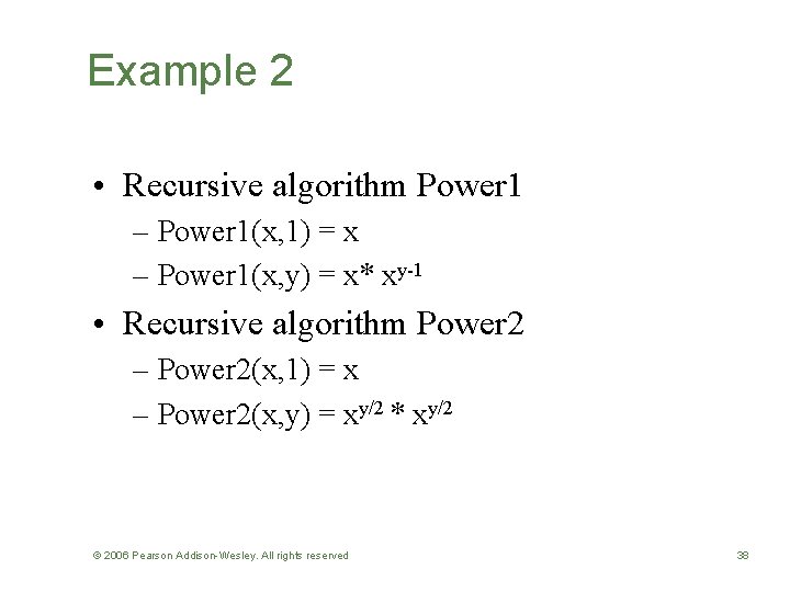
Example 2 • Recursive algorithm Power 1 – Power 1(x, 1) = x – Power 1(x, y) = x* xy-1 • Recursive algorithm Power 2 – Power 2(x, 1) = x – Power 2(x, y) = xy/2 * xy/2 © 2006 Pearson Addison-Wesley. All rights reserved 38

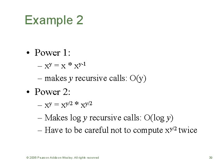
Example 2 • Power 1: – xy = x * xy-1 – makes y recursive calls: O(y) • Power 2: – xy = xy/2 * xy/2 – Makes log y recursive calls: O(log y) – Have to be careful not to compute xy/2 twice © 2006 Pearson Addison-Wesley. All rights reserved 39

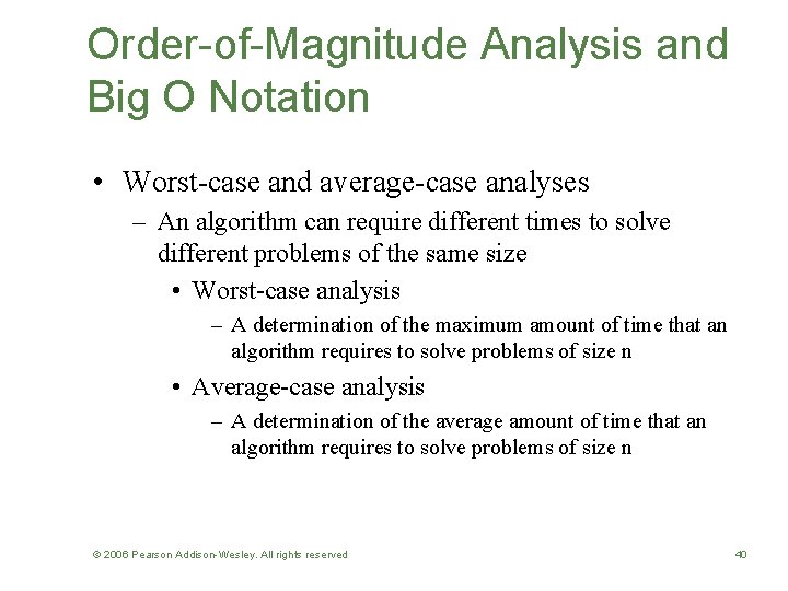
Order-of-Magnitude Analysis and Big O Notation • Worst-case and average-case analyses – An algorithm can require different times to solve different problems of the same size • Worst-case analysis – A determination of the maximum amount of time that an algorithm requires to solve problems of size n • Average-case analysis – A determination of the average amount of time that an algorithm requires to solve problems of size n © 2006 Pearson Addison-Wesley. All rights reserved 40

Keeping Your Perspective • Throughout the course of an analysis, keep in mind that you are interested only in significant differences in efficiency • Some seldom-used but critical operations must be efficient © 2006 Pearson Addison-Wesley. All rights reserved 41

Keeping Your Perspective • If the problem size is always small, you can probably ignore an algorithm’s efficiency • Weigh the trade-offs between an algorithm’s time requirements and its memory requirements • Compare algorithms for both style and efficiency • Order-of-magnitude analysis focuses on large problems © 2006 Pearson Addison-Wesley. All rights reserved 42