Module 2 2 Unconstrained Growth and Decay Angela

Module 2. 2 Unconstrained Growth and Decay Angela B. Shiflet and George W. Shiflet Wofford College © 2014 by Princeton University Press

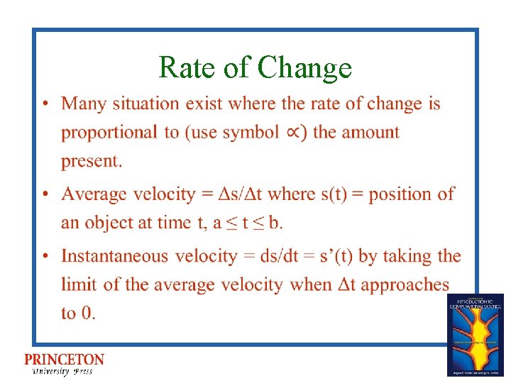
Rate of Change •

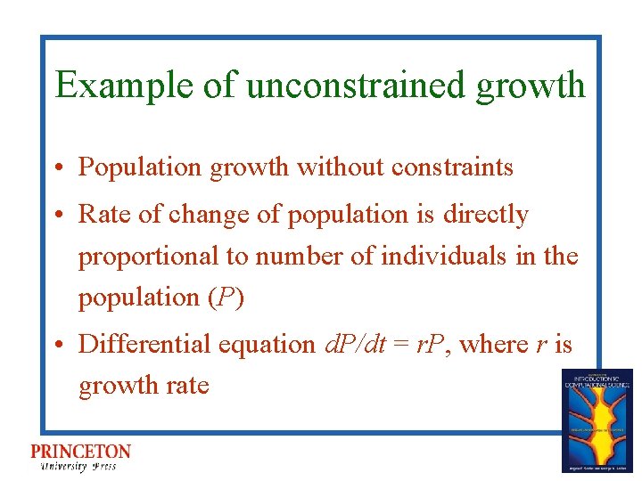
Example of unconstrained growth • Population growth without constraints • Rate of change of population is directly proportional to number of individuals in the population (P) • Differential equation d. P/dt = r. P, where r is growth rate

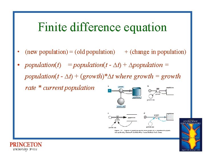
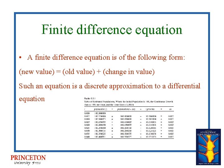
Finite difference equation • (new population) = (old population) + (change in population) • population(t) = population(t - ∆t) + ∆population = population(t - ∆t) + (growth)*∆t where growth = growth rate * current population

Finite difference equation • A finite difference equation is of the following form: (new value) = (old value) + (change in value) Such an equation is a discrete approximation to a differential equation

System's modeling tool • Helps to model • Performs simulation • What happens at one time step influences what happens at next

Stock/Box Variable/Reservoir • Anything that accumulates, buffer, resource • Examples • Population • Radioactivity • Phosphate • Body fat • Labor

Flow • Represents activities • Examples • Birthing, dying with population • Intaking & expending calories with body fat

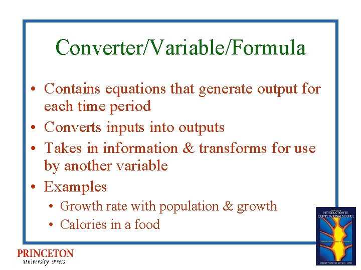
Converter/Variable/Formula • Contains equations that generate output for each time period • Converts inputs into outputs • Takes in information & transforms for use by another variable • Examples • Growth rate with population & growth • Calories in a food

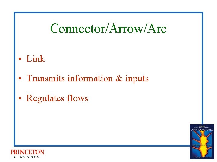
Connector/Arrow/Arc • Link • Transmits information & inputs • Regulates flows

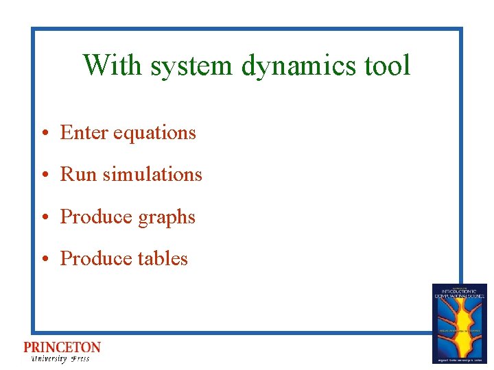
With system dynamics tool • Enter equations • Run simulations • Produce graphs • Produce tables

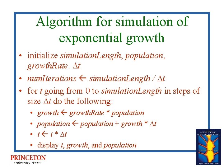
Algorithm for simulation of exponential growth • initialize simulation. Length, population, growth. Rate. ∆t • num. Iterations simulation. Length / ∆t • for t going from 0 to simulation. Length in steps of size ∆t do the following: • • growth. Rate * population + growth * ∆t t i * ∆t display t, growth, and population

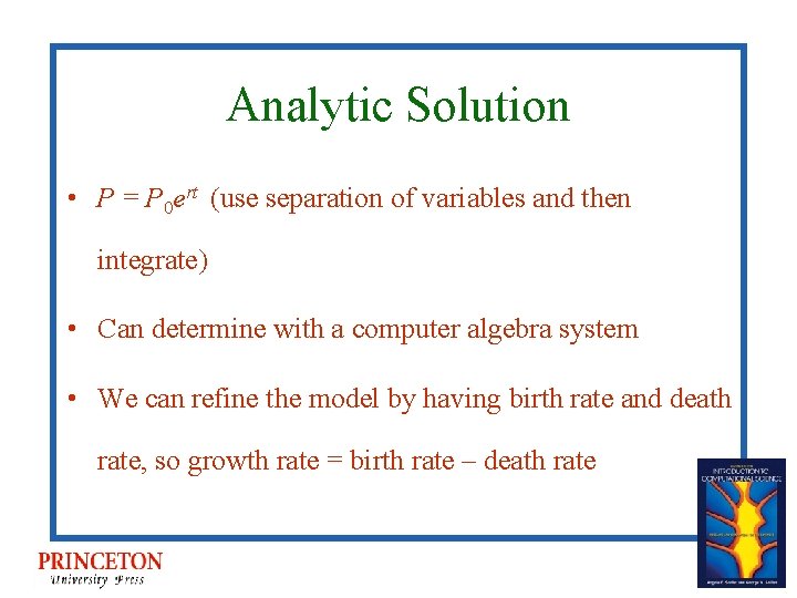
Analytic Solution • P = P 0 ert (use separation of variables and then integrate) • Can determine with a computer algebra system • We can refine the model by having birth rate and death rate, so growth rate = birth rate – death rate

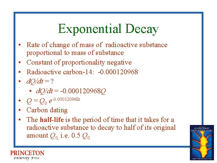
Exponential Decay • Rate of change of mass of radioactive substance proportional to mass of substance • Constant of proportionality negative • Radioactive carbon-14: -0. 000120968 • d. Q/dt = ? • d. Q/dt = -0. 000120968 Q • Q = Q 0 e-0. 000120968 t • Carbon dating • The half-life is the period of time that it takes for a radioactive substance to decay to half of its original amount Q 0, i. e. 0. 5 Q 0.

Quick Review Questions • Question 4 • Question 5