Luigi Calligaris CMS Pisa meeting 13012011 UPDATES ON

Luigi Calligaris CMS Pisa meeting 13/01/2011 UPDATES ON J/PSI POLARIZATION

Outline Data used for this analysis � Definiton of sidebands � Simulations on the contamination of the background by the signal, in the sidebands � PT dimuon distribution for different triggers � Cos θ and φ distributions in different reference frames of the positive muon �

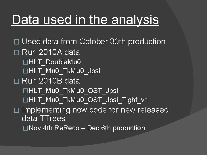
Data used in the analysis Used data from October 30 th production � Run 2010 A data � �HLT_Double. Mu 0 �HLT_Mu 0_Tk. Mu 0_Jpsi � Run 2010 B data �HLT_Mu 0_Tk. Mu 0_OST_Jpsi_Tight_v 1 � Implementing now code for new released data TTrees �Nov 4 th Re. Reco – Dec 6 th production

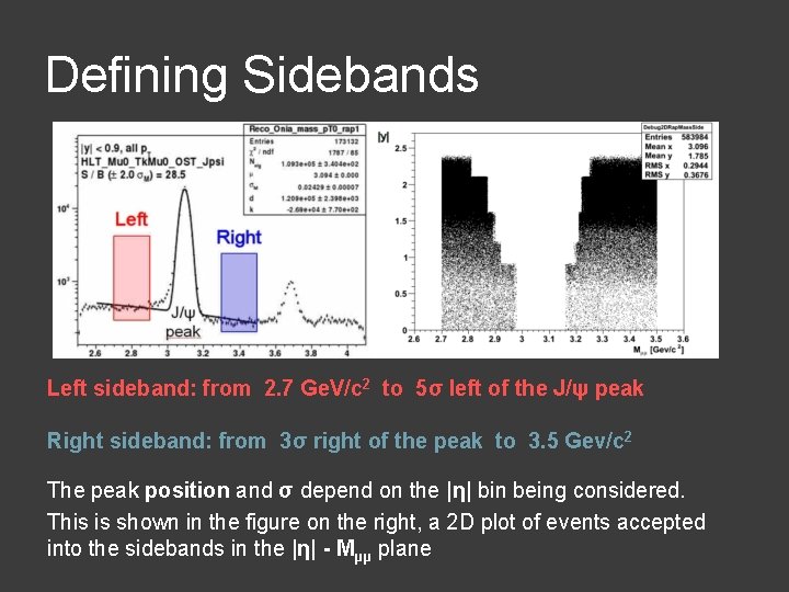
Defining Sidebands Left sideband: from 2. 7 Ge. V/c 2 to 5σ left of the J/ψ peak Right sideband: from 3σ right of the peak to 3. 5 Gev/c 2 The peak position and σ depend on the |η| bin being considered. This is shown in the figure on the right, a 2 D plot of events accepted into the sidebands in the |η| - Mμμ plane

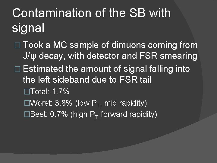
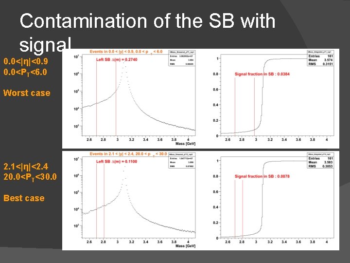
Contamination of the SB with signal � Took a MC sample of dimuons coming from J/ψ decay, with detector and FSR smearing � Estimated the amount of signal falling into the left sideband due to FSR tail �Total: 1. 7% �Worst: 3. 8% (low PT, mid rapidity) �Best: 0. 7% (high PT, forward rapidity)

Contamination of the SB with signal 0. 0<|η|<0. 9 0. 0<PT<6. 0 Worst case 2. 1<|η|<2. 4 20. 0<PT<30. 0 Best case

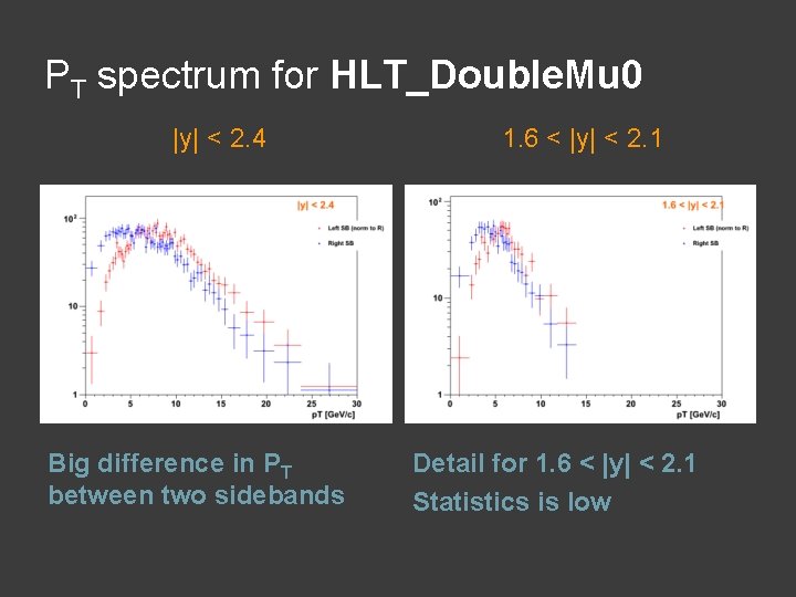
PT spectrum for HLT_Double. Mu 0 |y| < 2. 4 Big difference in PT between two sidebands 1. 6 < |y| < 2. 1 Detail for 1. 6 < |y| < 2. 1 Statistics is low

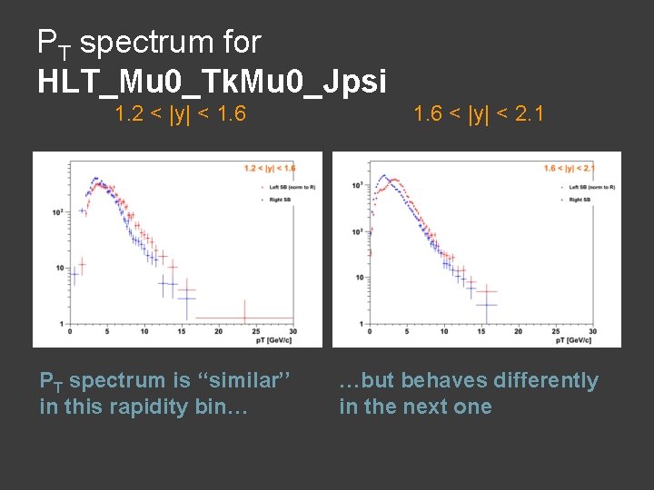
PT spectrum for HLT_Mu 0_Tk. Mu 0_Jpsi 1. 2 < |y| < 1. 6 PT spectrum is ‘‘similar’’ in this rapidity bin… 1. 6 < |y| < 2. 1 …but behaves differently in the next one

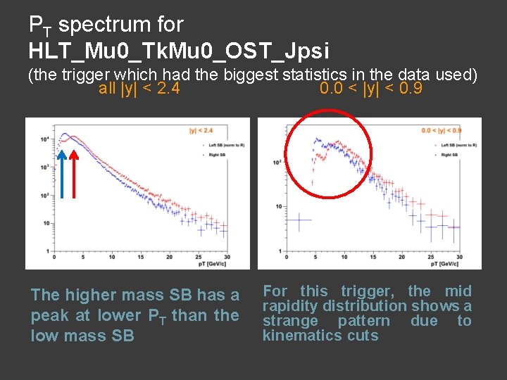
PT spectrum for HLT_Mu 0_Tk. Mu 0_OST_Jpsi (the trigger which had the biggest statistics in the data used) all |y| < 2. 4 0. 0 < |y| < 0. 9 The higher mass SB has a peak at lower PT than the low mass SB For this trigger, the mid rapidity distribution shows a strange pattern due to kinematics cuts

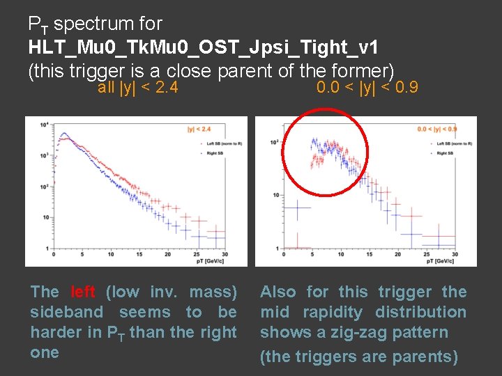
PT spectrum for HLT_Mu 0_Tk. Mu 0_OST_Jpsi_Tight_v 1 (this trigger is a close parent of the former) all |y| < 2. 4 0. 0 < |y| < 0. 9 The left (low inv. mass) sideband seems to be harder in PT than the right one Also for this trigger the mid rapidity distribution shows a zig-zag pattern (the triggers are parents)

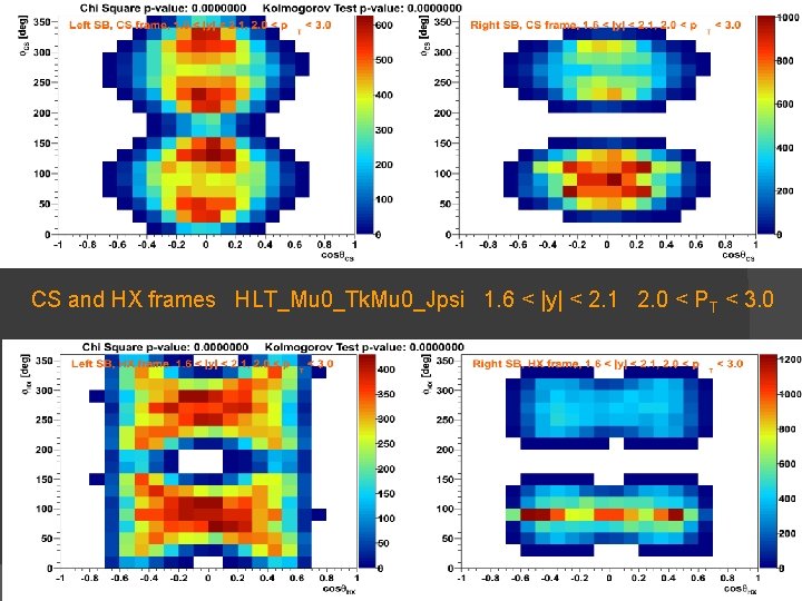
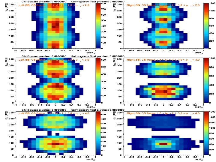
Cosθ and φ in different frames The following are 2 D plots of the Cosθ and φ of the positive muon in the dimouns considered, for different reference frames. � In the plots a cinematic dependence of the distribution in the two variables can be seen as we cycle trough different rapidity and PT bins. � Last but not least, there may be an effect due to ‘‘cowboy’’ dimuons inefficency. � I will show data for the trigger path for which we have the highest statistics: HLT_Mu 0_Tk. Mu 0_Jpsi �

CS and HX frames HLT_Mu 0_Tk. Mu 0_Jpsi 1. 6 < |y| < 2. 1 2. 0 < P T < 3. 0

HLT_Mu 0_Tk. Mu 0_Jpsi 1. 6 < |y| < 2. 1 2. 0 < PT < 3. 0

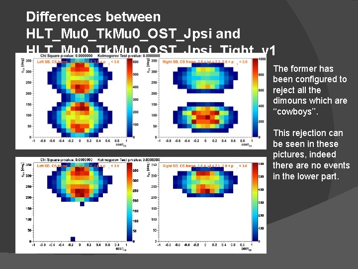
Differences between HLT_Mu 0_Tk. Mu 0_OST_Jpsi and HLT_Mu 0_Tk. Mu 0_OST_Jpsi_Tight_v 1 The former has been configured to reject all the dimouns which are ‘‘cowboys’’. This rejection can be seen in these pictures, indeed there are no events in the lower part.

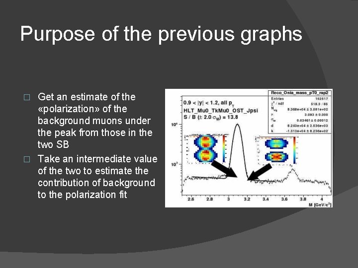
Purpose of the previous graphs Get an estimate of the «polarization» of the background muons under the peak from those in the two SB � Take an intermediate value of the two to estimate the contribution of background to the polarization fit �

Where to find more infos � QTF Workspace > Polarization > Data Quality Checks > Distributions from Mass Sidebands https: //espace. cern. ch/cms-quarkonia/onia-polarization/Data%20 Quality%20 Checks/Mass%20 sidebands. aspx � QTF Workspace > Polarization https: //espace. cern. ch/cms-quarkonia/onia-polarization/ � About reference frames and the analisys http: //arxiv. org/abs/1006. 2738 � ‘‘Seagulls and Cowboys’’ https: //espace. cern. ch/cms-quarkonia/upsilon/Lists/slides/Attachments/31/correlations_gavin_2010_05_10. pdf https: //espace. cern. ch/cms-quarkonia/onia-polarization/Lists/Meetings/Disp. Form. aspx? ID=39